Banding is not a bit depth
Assumes How bright is white and The midpoint is not half.
“Is eight bits enough?” is the question, and it has no answer. Not because the arithmetic is hard, but because a bit count is one of four things that decide whether a gradient bands, and it is the only one anybody writes down.

The claim
Whether a quantised gradient bands is decided by four quantities, and a bit depth is one of them. Computed on the same encoding, the same ramp length in code values and the same eight bits:
| where the ramp sits | steps | visibility |
|---|---|---|
| deep shadow, 0.02–0.2% of white | 11 | 58.6× threshold |
| shadow, 0.2–1% | 17 | 19.7× |
| lower midtone, 2–6% | 29 | 7.0× |
| mid grey, 16–24% | 23 | 2.8× |
| highlight, 50–80% | 45 | 1.5× |
A factor of forty in visibility, at one bit depth, from nothing but where in the tone scale the gradient lies.
The four quantities
How many code values the ramp crosses, which is what a bit depth sets. More bits, smaller steps, and the relationship is the obvious one.
Where in the tone scale it sits. The eye’s threshold is a contrast, so what matters is the code step divided by the local luminance. An sRGB code step near black is a Weber contrast of several per cent; near white it is a fraction of one.
How sharp each step is. A quantised ramp’s error is a sawtooth whose risers are one sample wide on a screen, and a sharp edge has energy at every frequency. This is the one everybody’s analysis gets wrong, and it is worth its own section below.
And how far away the reader is, which sets how many cycles per degree the bands occupy and therefore how much the eye’s own filter amplifies them.
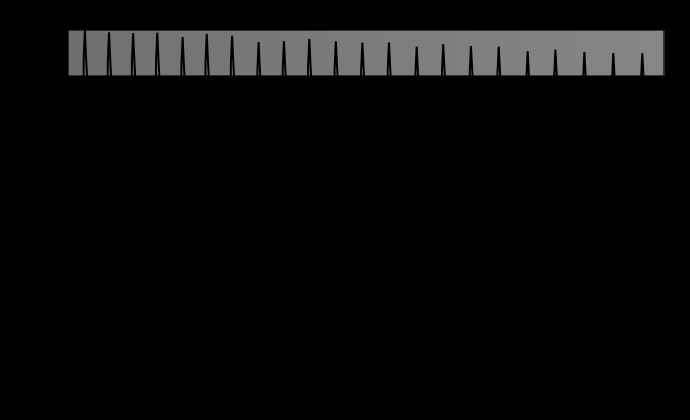
The same machinery on a pattern rather than a ramp says which part of the argument is about quantisation and which part is about the filter.

Bits, measured rather than assumed
| bit depth | shadow ramp | mid-grey ramp |
|---|---|---|
| 6 | 151× threshold | 11.6× |
| 8 | 29.8× | 2.8× |
| 10 | 5.8× | 0.54× |
| 12 | 1.4× | 0.13× |
Reading across: ten bits is enough at mid grey and not in the shadows. Twelve bits is marginal in the shadows — 1.4× threshold, which is visible under good conditions and not under ordinary ones.
That is precisely the finding that produced the PQ encoding: a transfer function whose code allocation follows a threshold model rather than a power law, so that the steps are equally invisible everywhere instead of being wasted at the top and short at the bottom. The row above is the argument for it, computed on the ordinary sRGB-shaped curve.
Each two bits buys a factor of about 4.6, which is close enough to four to be worth saying why. Two extra bits quarter the code step, and visibility is a filtered contrast, so if the edge’s shape were unchanged the response would fall by exactly four. It falls by 4.76 on the shadow ramp and 4.47 at mid grey, with the individual steps ranging from 4.14 to 5.19 — a scatter that is about where each riser happens to land relative to the sample grid, and a mean about fifteen per cent above the prediction.
So the finding two sections down does not disturb the scaling law: the risers stay one sample wide at every bit depth, so the shape of the error is unchanged and only its amplitude moves. The edge carries the visibility; the bit depth carries the amplitude; and the two are separable.
Which makes the table invertible, and the inversion is the number the question at the top of this essay actually wants. Taking 4.6 per two bits and asking what depth would put each row at threshold:
| where the ramp sits | at 8 bits | bits needed for invisibility |
|---|---|---|
| deep shadow, 0.02–0.2% of white | 58.6× | 13.3 |
| shadow, 0.2–1% | 19.7× | 11.9 |
| lower midtone, 2–6% | 7.0× | 10.5 |
| mid grey, 16–24% | 2.8× | 9.3 |
| highlight, 50–80% | 1.5× | 8.5 |
Thirteen and a third bits, on a power-law encoding, for the deepest gradient in the table — so fourteen, in a format that comes in whole bits. That is the honest answer to “is eight bits enough”, and it is also the clearest possible statement of why nobody ships fourteen-bit displays: the requirement is set by a region of the tone scale that a better-shaped transfer function makes cheap. Moving from a power law to a threshold-shaped curve does not add precision, it moves the precision that already exists from the highlight row — which needs 8.5 bits and is given the same allocation as everything else — to the shadow row that needs thirteen.
The edge carries it, not the band frequency
Here is the analysis everybody does, including the first version of this site’s machinery: the ramp has bands across degrees, so its fundamental is at cycles per degree; look up the sensitivity there and multiply by the step’s contrast.
That analysis says spreading a gradient over more degrees puts its fundamental at a lower frequency, where the eye is less sensitive, and therefore hides it. The measurement says the opposite:
| ramp width | measured visibility | fundamental-only estimate |
|---|---|---|
| 1° | 16.2× | 0.9× |
| 2° | 21.5× | 3.7× |
| 4° | 20.8× | 3.6× |
| 8° | 28.3× | 2.8× |
| 16° | 29.3× | 1.7× |
| 32° | 30.4× | 1.4× |
Both columns come from the same error signal. The left is its filtered response; the right is the amplitude of its fundamental times the sensitivity there.
The reason for the disagreement is that a staircase is not its fundamental. Each riser is a step of one code value happening across one sample, and a sharp step has energy at every frequency including the ones the eye is best at. Widening the ramp moves the fundamental down and leaves the risers exactly as sharp as they were, so the response rises with width and then flattens — which matches the everyday observation that wide, shallow gradients are where banding is met.
The right-hand column also says what the flattening is. Once the ramp is wide enough that consecutive risers are far apart in angle, each riser is an isolated edge, and the response to an isolated edge does not depend on how far away the next one is. So the left-hand column is converging to the visibility of one single-code-value step, about thirty times threshold for this ramp — and every wide gradient in the world converges to the same number.
That is the summary the model should be quoted by. “How visible is this gradient” depends on its width until it does not; “how visible is one step of this size at this luminance” is width-free, is what the wide cases all reach, and is the quantity a pipeline can actually be designed against. The first column reaches 96 per cent of its asymptote by eight degrees, so anything a reader would call a gradient is already in the width-free regime.
What dither does, and the half of it this model cannot explain
Dither is the standard repair: add noise before quantising so the staircase becomes something less structured.
Half of that story checks out immediately. Dither increases the error. Rounding a value that has had noise added to it is further from the truth, on average, than rounding the value: the root-mean-square error rises by 1.38× with high-passed noise and 1.44× with white.
The other half does not come out at all. In this model, both kinds of dither leave the filtered response the same or worse — 1.00× for high-passed noise and 0.58× for white, on five ramps out of five. The model says dither is not an improvement, and the textbook says it is, and the textbook is right about screens.
What is missing is stated rather than patched. The advantage of a dither mask rests on two things this model does not have:
- A second spatial dimension. A mask’s power spreads into an annulus at high radial frequency, while a band edge stays a straight line; a one-dimensional model sees a slice through that and misses the geometry entirely.
- A nonlinearity. A coherent edge is more visible than incoherent noise of the same contrast, which is masking, and a linear filter cannot express a preference between them.
So assertDitherIsNotExplainedHere requires the effect to stay absent. If a future revision starts predicting that dither helps, the build stops and somebody reads why — the same shape as the Stevens effect’s absence and the appearance model’s missing Helmholtz–Kohlrausch term. A model that quietly starts agreeing with a claim it has not earned is worse than one that openly disagrees.

What the room does to the same ramp
There is a fifth quantity, and it is the one nobody controls: the room.
Ambient light reflected off a screen adds a constant to every luminance. That lifts the black floor — a 1000:1 panel at 300 lux is a 137:1 panel — and lifting the floor is exactly what makes a shadow ramp safer, because a code step near black becomes a smaller fraction of a larger local luminance. The room that ruins the contrast ratio rescues the banding.
The direction is worth stating plainly because it inverts the usual advice. A dark viewing environment is better for contrast and worse for quantisation, and a colourist grading in a black room is working in the conditions where the shadows band most.

What was computed, and how
The ramp is built in luminance across the stated angular width at the screen’s own sample rate, encoded with a power-law transfer function, quantised to the stated depth, and decoded.
The error is the difference between the quantised and ideal luminances, expressed as a Weber contrast against the local ideal — — because that is the form the threshold is stated in and is the whole reason the shadow end behaves differently from the highlight end.
The response is that error signal passed through the luminance contrast sensitivity function, normalised so its peak is unit gain, and the reported figure is the largest response divided by the threshold contrast of 0.003. A ratio above one is a prediction that the banding is visible.
The dither is a deterministic generator, so the figure is identical on every build, in two forms: white noise of half a code value, and the same noise high-passed by subtracting a three-sample local mean and rescaled to identical power. Identical power, different placement, which is what a dither mask is.
And the geometry is stated: 41 pixels per degree, a reader 60 cm from a display of about a hundred pixels to the inch.
Where the model stops
One dimension, which is what makes the dither result a null rather than a finding.
One transfer function. Everything above is a 2.2 power law. PQ, HLG and a log curve allocate code values differently and would change every row; the machinery would take them and this essay does not.
A stated threshold with a wide range. The 0.003 anchor is reported between 0.002 and 0.005, so every “times threshold” figure carries a factor of about 1.7 in either direction. What survives that uncertainty is the ratios between rows, which share the anchor.
No temporal dimension, so nothing here says anything about the moving version of the same artefact, which is what a video codec actually has to manage.
And no chroma. The ramp is neutral. A gradient between two saturated colours quantises in three channels at once, and the resulting error is a coloured mottling rather than a set of grey steps — and the eye’s chromatic channels are much worse at seeing it, which is why chroma banding is a smaller problem than the bit counts suggest.
The generalisation
A quantisation error is a signal, and whether it is visible is a question about the signal rather than about the quantiser.
Bits per channel is a property of a file. Visibility is a property of a file, a transfer function, a tone range, a display, a viewing distance and an eye — and the practice of specifying the first alone is the same mistake as specifying a lamp by its colour temperature or a colour by three numbers with no observer: a summary that closed over the wrong operations.
The version of this that generalises furthest is about where a number’s precision is spent. Every encoding is an allocation of a fixed number of code values across a range, and the good ones follow a threshold model — which is why PQ exists, why companded audio exists, and why a linear-light image format needs more bits than anybody expects. The bad ones are uniform in a quantity nobody perceives uniformly.
Who found it, and when
Contouring in quantised images is as old as digital imaging, and the arithmetic connecting it to contrast thresholds dates from the 1960s and 1970s, when the question was how many bits a broadcast frame store needed.
Dither is older still — as a deliberate technique it goes back to wartime analogue computing, and the modern account of it is Roberts’s, in 1962, in exactly this setting: adding noise before quantising an image so that the error stops being structured. Blue-noise masks, which put the noise where the eye is worst, are Ulichney’s from the late 1980s.
The most recent chapter is the display standards. Ten and twelve bit encodings with threshold-shaped transfer functions were adopted for high dynamic range for exactly the reason in the table above: at ordinary bit depths and a power-law curve, the shadows band and everything above mid grey has precision to spare.
What the pictures cannot show
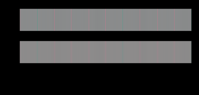
Whether the reader’s own screen bands. Every figure here is drawn as a set of computed swatches at stated luminances, rendered through the reader’s transfer function on the reader’s panel at the reader’s brightness setting. A ten-bit panel and an eight-bit one showing the same page differ in exactly the quantity being discussed, and the page cannot tell which it is on.
And the strips are drawn coarser than they are computed. The ramp figures compute at the screen’s own sample rate — several hundred points across twelve degrees — and draw a hundred and eighty cells, because a rectangle per computed sample cost fifty kilobytes on a figure whose argument is entirely in the curve below it. The curve is the measurement; the strip is an illustration of it.
The rule that falls out
Do not ask how many bits. Ask what the darkest gradient in the content is, how wide it is drawn, and what the encoding is.
For an ordinary power-law encoding, the table above says eight bits is comfortable above about a fifth of white, marginal in the lower midtones and hopeless below a hundredth. Ten bits moves each of those boundaries down by roughly a factor of ten in luminance, which is exactly what a factor of four in code values buys against a curve of this shape.
The inverted table sharpens that into a rule of thumb worth carrying, because the spacing between its rows is nearly constant: each decade darker costs about a bit and a half. Mid grey wants 9.3, the lower midtone 10.5, the shadow 11.9, the deep shadow 13.3 — four rows about a decade apart in luminance and about 1.4 bits apart in requirement. So the question “how many bits” reduces to “how dark”, and the conversion is one number.
It also explains why the argument is usually conducted at cross purposes. Somebody defending eight bits is thinking about the rows near the bottom of that table, where eight is genuinely comfortable, and somebody attacking it is thinking about the rows near the top — and both are right about the content they have in mind. A decade and a half of luminance separates the two positions, which is nothing at all in a picture that contains both a sky and a shadow.
And the content is the argument nobody has. A picture with no smooth dark gradient in it does not band at eight bits; a picture that is mostly a dark sky does at ten. That is a statement about what is being shown rather than about the pipeline showing it, and it is the reason bit-depth arguments never converge.
Where the ladder goes next
The two-dimensional model is the obvious next step and the one that would turn the dither null into a result. Everything else in the machinery would carry over; the cost is that a two-dimensional filter over an image is a much heavier computation and a much heavier figure.
The second is chroma. The whole of this essay is a neutral ramp, and the interesting practical case — banding in a sky, in a skin tone, in a gradient between two brand colours — is a three-channel quantisation whose error has a chromatic direction. The channels differ by a factor of six in what they can resolve, so the visibility of a chroma band is a different calculation with the same parts, and this phase has both halves and has not joined them.
Where this goes next
 How bright is white
An sRGB value says a pixel is some fraction of whatever the display can manage. A PQ value says it is two hundred candelas. The change is the largest in display encoding since gamma, and what it removed was the honest admission that nobody knew.
How bright is white
An sRGB value says a pixel is some fraction of whatever the display can manage. A PQ value says it is two hundred candelas. The change is the largest in display encoding since gamma, and what it removed was the honest admission that nobody knew.
 The midpoint is not half
Code 128 sits halfway along the sRGB scale and carries about a fifth of white's luminance. Half the luminance is code 188. Almost every gradient, blur and resize on the web gets this wrong, and the errors are visible once known.
The midpoint is not half
Code 128 sits halfway along the sRGB scale and carries about a fifth of white's luminance. Half the luminance is code 188. Almost every gradient, blur and resize on the web gets this wrong, and the errors are visible once known.
 A difference has no size
A colour difference formula answers a question about two large patches seen side by side. Applied to a pattern, it reports fourteen units where the eye is left with less than one — and the ratio depends on nothing but how finely the difference is spread.
A difference has no size
A colour difference formula answers a question about two large patches seen side by side. Applied to a pattern, it reports fourteen units where the eye is left with less than one — and the ratio depends on nothing but how finely the difference is spread.
What this makes readable
Essays that name this one as a prerequisite.
Named alongside this one
Essays reaching for the same objects. Nobody chose these; they are what the index of named objects makes visible.
- The list nobody made banding · contrast sensitivity · dither · quantisation · spatial frequency · threshold
- A halftone is a luminance object contrast sensitivity · spatial frequency · threshold · viewing distance
- A tint at the edge of a page contrast sensitivity · spatial frequency · threshold · viewing distance
- The eye counts a corner's error, not its peak contrast sensitivity · spatial frequency · transfer function · viewing distance
- What a still eye stops seeing contrast sensitivity · spatial frequency · threshold · viewing distance
- A fading pool has a shape contrast sensitivity · spatial frequency · threshold
What links here
The 8 essays that link to this one and share the most of its objects, of 17 that link here.
The objects this essay names
Each one links to every other essay that touches it.
BandingContrast sensitivityDitherDynamic rangeEncodingQuantisationSpatial frequencyThresholdTransfer functionViewing distance