The list nobody made
Assumes Every threshold was measured with a grating and Banding is not a bit depth.
The previous phase ended with a rule and an admission. The rule: a model inherits the question its measurements were made with. Every threshold under this site’s spatial machinery was measured with a grating, so the model is a statement about components, and reading it at a point in space asks it something it was never fitted to.
The admission was that nobody had gone back through the site to see which claims that touched. This is that list, and the rule does not survive it in the form it was written.

What it would cost to hand the second reading to a reader rather than print it is the other half of the same ledger, and it is a number in bytes.

The claim
The rule is right in one direction and wrong in the other.
- Every comparison with noise on one side of it moves, by a lot. A blue-noise mask against a plain ramp reads 0.40 at a point and 14.4 as components — a factor of 35.6, and the two readings disagree about the direction of the effect. White noise, 38.4. A halftone screen against a noise field of the same mean, 111.
- But two comparisons between two structured fields move as well. The same ramp in the shadows against the same ramp at mid grey reads 4.88 at a point and 1.46 as components. One screen coverage against another reads 0.59 and 1.89 — a reversal.
- So noise is sufficient and not necessary. The narrower statement the table supports is that the two readings agree only when the two fields differ in amplitude. Whenever they differ in where their energy sits, the readings are asking different questions and get different answers.
What a reading is
The point reading is the largest absolute departure anywhere in the field, weighted by the eye’s filter: what somebody would get by hunting for the worst pixel.
The component reading is the largest single spatial frequency surviving the same filter, which is the quantity every threshold underneath was measured as. A contrast sensitivity function is a curve of threshold against spatial frequency; it was obtained by showing observers sinusoidal gratings and asking when they could see them; and its natural argument is therefore a Fourier component and not a location.
Both come out of the same call. Nothing in this file re-derives any physics: it arranges existing measurements and takes ratios.
And that is the point of doing it as a table rather than as an essay per claim. A rule about which comparisons are affected can only be checked against a set of comparisons, and a set means seven claims read the same way by the same code, not seven essays each making its own argument.


The seven
Dither, blue noise against a plain ramp. Point 0.40, components 14.4. The plain ramp’s worst departure is at a quantisation edge; the dithered version’s worst departure is somewhere in the noise and is larger. Read as components the noise’s energy is at high frequencies the eye discards and the ramp’s is at low ones it does not, so the answer inverts. This is the previous phase’s worked example and the largest reversal in the table.
Dither, white noise. Point 0.33, components 12.5. Same structure, slightly smaller, because white noise puts energy everywhere rather than only where the eye is worst.
Bit depth, eight against ten. Point 4.12, components 5.88 — a ratio of 1.43, the only claim in the table that agrees. Two ramps at different quantisations have the same shape of error and differ mostly in amplitude, which is precisely the condition under which a point reading and a component reading track each other.
Ramp position, shadows against mid grey. Point 4.88, components 1.46 — a ratio of 0.30, and no noise anywhere in it. A ramp in the shadows has larger, more widely spaced steps than one at mid grey, so the two differ in the frequency of their step structure and not only in its size. The point reading, which finds the tallest step, reports a factor of five; the component reading, which asks which frequency survives the filter, reports a factor of one and a half.
Screen angle, 0° against 45°. Point 1.28, components 0.98 — and a reversal, though a small one. The site’s screen-angle essay reports a factor of two for a real ruling, computed harmonically; asked at a coarse ruling that a raster can represent, the point reading says the cardinal screen is louder and the component reading says the two are equal. That is a warning about the essay’s number rather than a refutation of it: the screen-angle claim is a component claim by necessity, because a real screen is past the Nyquist frequency of any field small enough to compute.
Screen coverage, half against a fifth. Point 0.59, components 1.89 — a reversal, no noise. Two coverages produce different harmonic content, not merely different amounts of the same content, so the two readings order them oppositely.
A screen against a noise field of the same mean. Point 28.5, components 3,165 — a ratio of 111, the largest in the table and the one that best shows the mechanism. A screen’s energy is concentrated at four points in the frequency plane; a noise field’s is spread over the whole of it. A point reading compares two maxima in space; a component reading compares a spike against a floor.
What the corrected rule is
The previous phase said: comparisons with noise on one side of them move. That is confirmed and strengthened — every noisy comparison here moves by at least 35 times, and the gap to the largest structured mover is a factor of eleven with nothing in it.
What is false is the converse. Two structured comparisons move by 3.2× and 0.3×, and two of the four structured comparisons reverse direction.
The rule that fits all seven is: a point reading and a component reading agree when the two fields differ in amplitude, and diverge when they differ in where their energy sits.
Noise is the extreme case of differing in where the energy sits — a noise field’s spectrum is as unlike a ramp’s or a screen’s as two spectra can be — which is why the noisy comparisons are the large ones and why the original rule found them first. But a ramp in the shadows and a ramp at mid grey differ in their step frequency, and one screen coverage differs from another in its harmonic weights, and neither of those has any noise in it.
This is a correction to a rule this site published one phase ago, and it belongs beside the measurement rather than in a footnote. The previous phase’s rule would have told an author that a comparison between two halftone screens was safe to read either way. It is not.
What was computed, and how
Each claim is one function returning two numbers, from the same underlying call: bandingVisibility2d already reports a peak in space and a peak component, and screenVisibility reports a peak alongside the field it was computed from, whose transform gives the component. Nothing is recomputed and nothing is fitted.
noisy is declared, not detected. Whether a field is a noise field is a fact about how it was built, and no measurement decides it — a mask is noise by construction and a halftone screen is not. Declaring it is what makes the rule testable: if the flag were derived from the same data the rule is being tested on, the test would be circular.
The verdict thresholds are stated. A claim “disagrees” when the ratio between the two readings exceeds one and a half in either direction, and “reverses” when the two readings fall on opposite sides of one — which is the stronger property, and four of the seven have it.
And the assertions are written to fail in both directions. assertTheAuditIsNotEmpty requires that some claims disagree and that not all of them do, because a table in which everything moves is as uninformative as one in which nothing does.
Where the model stops
Seven claims is not the site. These are the filtered claims that report both readings from one call. Others — the colour difference spread as a pattern, the chroma subsampling result, the peripheral tint — would each need their own two readings written, and the ones with a noise field on one side are the ones to write first.
The two readings are not the only two. A root-mean-square over the field is a third, an image-difference metric filtered through a spatial model is a fourth — and which statistic is chosen decides the ranking — and a real observer’s report is a fifth that none of them approximates well. What the table establishes is that the choice matters, not that either of these two is right — the same conclusion a tolerance stated in the wrong coordinates arrives at from the other side.
And the point reading is a strawman in one specific sense. Nobody hunting for the worst pixel is doing psychophysics; they are doing quality control. The reason the point reading appears in this site’s essays at all is that a peak over a field is the natural thing to compute when a field is what the code has, and it is a defensible statistic — just not the statistic the thresholds underneath it were measured with.
The generalisation
The sentence worth carrying is: a model answers the question its measurements were phrased in, and every other question it is asked is an extrapolation.
That is the same rule generalised past spatial vision, and this site’s own history is full of it. The colour difference formulae were fitted on suprathreshold judgements and are quoted as thresholds. The appearance model was fitted on settled states and is asked about instants. The standard observer was fitted on colour matches and is asked about appearance.
In each case the extrapolation is not obviously wrong and is not obviously right, and the size of the error is measurable only by doing what this essay does: computing the same claim both ways and looking at the ratio.
The surprising part is how often the two ways disagree about the sign. Four of seven claims here reverse. That is not a small correction to a magnitude; it is a different conclusion. An author reading a filtered field at a point and reporting that dither makes things worse is not making a rounding error — they are reporting the opposite of what the thresholds underneath the model support.
Who found it, and when
The grating tradition in spatial vision starts with Schade in the 1950s and Campbell and Robson in 1968, whose whole contribution was to treat the visual system as a set of channels tuned to spatial frequency and to measure it with sinusoids. Everything downstream of that inherits the sinusoid.
The alternative tradition — measuring detection of edges, points and real images — exists and is smaller, partly because the results are harder to generalise: an edge has a spectrum, so an edge threshold is a weighted sum over channels rather than a channel measurement, and inverting the sum needs the channels anyway.
The point at which the two are conflated is not in the literature; it is in every implementation. Given a field and a filter, the natural thing to compute is a filtered field and then take a maximum, and every graphics or imaging library that offers a contrast sensitivity function offers it as something to multiply a spectrum by, leaving what to do afterwards to the caller.
And this site conflated them for two phases before noticing, which is the honest note to end the history on. The rule that caught it was written a phase ago; the list confirming and correcting it is here; and what neither of them would have found without a table is that the rule as first stated was too narrow.
What the pictures cannot show
They cannot show a reading. A point reading and a component reading are two ways of summarising the same picture, and a figure of the picture shows neither — which is why this essay’s figures are bars and ratios rather than fields.
And the table cannot show what a person would report. Neither reading is a measurement of a viewer; both are summaries of a model, and the model’s thresholds came from experiments in one of the two frames. What a person hunting a printed sheet for defects reports is probably closer to the point reading, and what a person glancing at a page is probably closer to the component one, and this site has no way to settle it.
The two verdicts are independent, and the table proves it four ways
The verdicts stated above are that a claim disagrees when the ratio between its two readings leaves the band from 1/1.5 to 1.5, and reverses when the two readings fall on opposite sides of one — with reversal described as the stronger property. Applied to the seven rows, that description does not hold, and the table is the reason.
| claim | ratio | departure | disagrees | reverses |
|---|---|---|---|---|
| blue noise | 36.0 | 36.0 | yes | yes |
| white noise | 37.9 | 37.9 | yes | yes |
| bit depth, 8 against 10 | 1.43 | 1.43 | no | no |
| ramp position | 0.299 | 3.34 | yes | no |
| screen angle | 0.766 | 1.31 | no | yes |
| screen coverage | 3.20 | 3.20 | yes | yes |
| screen against noise | 111 | 111 | yes | no |
All four combinations appear, which is what independence looks like. Screen angle reverses without disagreeing — its two readings are 31 per cent apart, comfortably inside the band, and they still land on opposite sides of one because both sit close to it. Screen against noise disagrees by a factor of 111 without reversing, because both readings are far above one and the question of which side they are on never arises. Reversal is not a stronger form of disagreement; it is a different question, about proximity to unity rather than about separation.
That corrects a count as well. The bit-depth row is described above as the only claim in the table that agrees, and by the threshold the essay itself states there are two: screen angle at 1.31 is inside the band with it. What distinguishes them is not agreement — both agree — but that one pair straddles unity and the other does not.
And the corrected rule needs one more word
The rule the seven rows are used to establish is that the two readings agree when the fields differ in amplitude and diverge when they differ in where their energy sits. The screen-angle row is a counterexample to that as written, and repairing it is worth more than the repair.
Two screens at 0° and 45° differ in nothing but where their energy sits: the four spikes are in the same places at a different rotation. By the rule, that comparison should be among the largest movers. It is the second smallest, at 1.31, and the component reading reports the two screens as very nearly equal.
The reason is that the filter the readings are weighted by takes a radial frequency, and a rotation moves energy around the plane without moving it along the radius. A component reading is therefore blind to orientation by construction, and the point reading is not — which is precisely why the two land on opposite sides of one, and why the screen-angle essay’s factor of two has to be a component claim computed harmonically rather than anything a coarse raster can be asked.
So the rule wants a qualifier: the two readings diverge when the fields differ in where their energy sits along the argument the filter is a function of. Radial frequency, here. Energy moved anywhere else — around the plane, between orientations — is invisible to the component reading and visible to the point reading, and that produces a reversal at small magnitude rather than a disagreement at large one, which is exactly the pattern the screen-angle row has.
This is a correction to a correction, and the sequence is the honest record: a rule was published, a table was built to check it, the table said the rule was too narrow, and reading the table’s own verdict columns says the widened rule is too broad in one specific place. Three revisions is not a sign that the machinery is unreliable — it is what happens when each statement is given a test it could fail, and the screen-angle row failed two of them.
Where the ladder goes next
The nearest unfinished piece is extending the table. Three claims elsewhere on the site have noise on one side of them and have never been read as components, and by this table’s rule all three will move by more than an order of magnitude.
The second is the third reading. Neither a peak in space nor a peak in frequency is what an image-difference metric computes: those filter first and then pool, usually with an exponent between two and infinity — and a mean and a worst case are two specifications — and the exponent is where the disagreement between these two readings lives. Adding one pooled reading to the table would put the two extremes in context and might collapse the disagreement entirely.
And the third is a gate rather than an essay. Nothing in this site’s machinery records which reading an essay’s number came from, so the next author to filter a field has nothing to check against. A rule that has now been corrected once is a rule worth enforcing rather than remembering.
Where this goes next
 Every threshold was measured with a grating
An earlier essay here claimed that the model cannot explain why dither works, and named two missing pieces. One of them was real and worth thirteen times the guess; the other was not needed. The piece nobody named was the detector — and reading the same model two ways changes the answer by a factor of fifty.
Every threshold was measured with a grating
An earlier essay here claimed that the model cannot explain why dither works, and named two missing pieces. One of them was real and worth thirteen times the guess; the other was not needed. The piece nobody named was the detector — and reading the same model two ways changes the answer by a factor of fifty.
 Banding is not a bit depth
Eight bits bands at thirty times threshold in the shadows and at under three at mid grey, on the same ramp with the same encoding. What decides is where in the tone scale the gradient sits, how sharp each step's edge is, and how far away the reader is — and a bit count contains none of the three.
Banding is not a bit depth
Eight bits bands at thirty times threshold in the shadows and at under three at mid grey, on the same ramp with the same encoding. What decides is where in the tone scale the gradient sits, how sharp each step's edge is, and how far away the reader is — and a bit count contains none of the three.
 A pattern has a direction
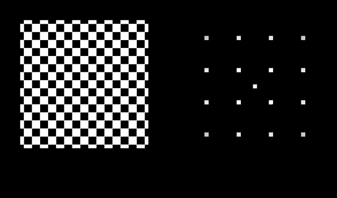
Every spatial claim here is a claim about a frequency, and a frequency has no direction in it. Turning a printed screen forty-five degrees makes it exactly twice as quiet with nothing else changed — and the same rotation does nothing at all to a chromatic one.
A pattern has a direction
Every spatial claim here is a claim about a frequency, and a frequency has no direction in it. Turning a printed screen forty-five degrees makes it exactly twice as quiet with nothing else changed — and the same rotation does nothing at all to a chromatic one.
What this makes readable
Essays that name this one as a prerequisite.
Named alongside this one
Essays reaching for the same objects. Nobody chose these; they are what the index of named objects makes visible.
- A tint at the edge of a page contrast sensitivity · halftone · image difference · sampling · screen angle · spatial frequency · threshold
- A halftone is a luminance object contrast sensitivity · halftone · screen angle · spatial frequency · threshold
- A fading pool has a shape assertion · contrast sensitivity · spatial frequency · threshold
- How fine a colour edge can be contrast sensitivity · image difference · sampling · spatial frequency
- The drift is a luminance mechanism assertion · contrast sensitivity · spatial frequency · threshold
- What a still eye stops seeing assertion · contrast sensitivity · spatial frequency · threshold
What links here
Every essay whose body links to this one.
The objects this essay names
Each one links to every other essay that touches it.
AssertionBandingContrast sensitivityDitherHalftoneImage differenceMeasurement errorQuantisationSamplingScreen angleSpatial frequencyThreshold