Concept

Sampling — where it appears

Recording a continuous thing at discrete points, after which what happens between them is a choice rather than a measurement. The interval and the bandwidth are separate decisions and both are stated, because a coarse interval and a wide slit lose different things.

Named by 36 essays across 8 fields — each of them below, with the objects they name alongside it.

A grey edge, reconstructed from a Bayer row, arrives coloured. Above: an achromatic step through 24 sensor sites, with green sampled on the even ones and red on the odd. Interpolating each channel separately reconstructs them from data taken on either side of the edge, so their ratio moves. Below: the resulting chroma, peaking at 144 per cent of the local mean, and 112 per cent once colour differences are interpolated instead.

A grey edge arrives coloured

A sensor site measures one channel and the other two are interpolated from neighbours that sat somewhere else. Across a black-and-white step that reconstruction gives an achromatic scene a chroma of 144 per cent of its own local mean, and nothing in the scene or the sensor was coloured.
imaging · Capture
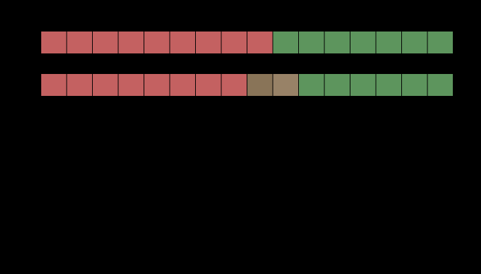
An edge at 4:2:2, and the colour it arrives as. Above, the row as it was sent and as it arrives after the two chroma planes are averaged 2 samples at a time. Below, the colour difference at each sample. The worst is ΔE00 = 25.88, at a luma step of 0.058 across the edge — an edge of nearly equal luminance. Nothing is wrong with the codec: it discards the differences the eye resolves worst, and this edge is made of nothing else.

Colour thrown away on purpose

Every video format in use discards three quarters of its colour information and keeps all of its luminance, because the eye resolves fine colour detail badly. On an edge that carries luminance the loss is exactly zero. On an edge of nearly equal luminance it is a colour difference of forty-three, and the two edges are the same edge to the codec.

applied · Delivery
Contrast sensitivity, three channels, normalised to each channel's peak. Spatial frequency in cycles per degree against relative sensitivity. The luminance channel runs to 50 cycles per degree, red–green to 12 and blue–yellow to 8, each by the same criterion of 5 per cent of that channel's own peak. Only the luminance channel dips at low frequency; the two chromatic ones are low-pass, so a chromatic edge of any size at all is seen at its full contrast.

How fine a colour edge can be

The eye resolves a lightness pattern to about fifty cycles per degree and a red–green one to twelve. Every colour difference here is quoted as though a patch had no size, and the same difference is plainly visible at one scale and gone at another.

eye · Cones
What a coarse wavelength grid costs, by source. Colour error against grid size, for four sources through one reflectance. Daylight survives every grid tested: 0.67 ΔE00 even at 40 nm. A source with lines in it does not — the narrowband source reaches 16.2. The grid is not a property of the arithmetic; it is a claim about what the light has in it.

Five nanometres is a choice

Every integral here is taken in five-nanometre steps, and the interval has never had to be defended. Coarsening it to twenty costs daylight two hundredths of a colour difference and a fluorescent tube six and a half — and which way of coarsening is used decides a further factor of six.
matching · Gamut
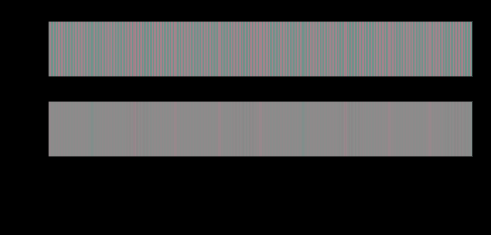
A chromatic line screen at 10.0 cycles per degree. The upper strip is the pattern as delivered and the lower one is the same pattern after each opponent channel has been low-passed at its own cutoff. Against a flat field of the same mean, the delivered pattern differs by up to ΔE00 14.22 and the filtered one by 7.77 — a ratio of 1.8. Every number quoted elsewhere for a difference of this kind is the first one.

A difference has no size

A colour difference formula answers a question about two large patches seen side by side. Applied to a pattern, it reports fourteen units where the eye is left with less than one — and the ratio depends on nothing but how finely the difference is spread.
difference · Metric
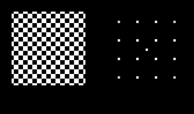
A screen at 45°, 8 c/°, and where its energy sits. Left, the pattern. Right, its power in the frequency plane with the zero frequency at the centre and the edges at the sampling limit of 23 cycles per degree, on a logarithmic scale over five decades. The closed curves are the visual system's own sensitivity at 5, 25, 60 per cent of its peak; they are not circles, because sensitivity is lower on the diagonals than on the cardinal axes by a factor of 2.0 at high frequency. Energy inside a curve is seen; energy outside it is not, whatever its size.

A pattern has a direction

Every spatial claim here is a claim about a frequency, and a frequency has no direction in it. Turning a printed screen forty-five degrees makes it exactly twice as quiet with nothing else changed — and the same rotation does nothing at all to a chromatic one.

eye · Cones
What a dither mask is worth, read as components, in two dimensions. Five luminance ramps, each quantised to 8 bits with and without a high-passed mask of the same power. The bars are the most visible single sinusoidal component of the error, as a multiple of the contrast that component needs to be seen: above the line at one it is visible. The mask lowers it by 20–22×, on every ramp — which the one-dimensional model on this site says it does not, and that disagreement is the finding.

Every threshold was measured with a grating

An earlier essay here claimed that the model cannot explain why dither works, and named two missing pieces. One of them was real and worth thirteen times the guess; the other was not needed. The piece nobody named was the detector — and reading the same model two ways changes the answer by a factor of fifty.

limits · Limits
A halftone tint away from the centre of gaze, two ways. The upper curve raises the threshold by the E2 rule and leaves the filter alone, which is the multiplication the last phase guessed at. The lower one also moves the cutoff, because eccentricity magnifies the whole spatial scale — implemented as the substitution that makes it exact, a screen of ruling r seen through a filter whose cutoff has been divided by s being a screen of ruling r·s seen at the fovea. The horizontal line is threshold. The screen is visible where you are looking and gone by 3°, while the product prediction has it visible across the whole page.

A tint at the edge of a page

The last phase left this join open and guessed at its answer — how visible a halftone tint is away from the centre of gaze should be the product of two effects it had measured separately. It is not the product. At five degrees the guess is fifty-three times too generous, and by twenty it is out by eight orders of magnitude.

difference · Metric
Every filtered claim in these essays, read at a point and read as components. Each row is a comparison one of the essays makes. The bar is the ratio between the two readings — how many times larger the component answer is than the point answer, or the reverse — on a logarithmic scale. 5 of 7 disagree by more than half again, and 4 disagree about the direction of the effect rather than merely its size. The three marked as noisy are the ones with a noise field on one side of the comparison, and they are the three largest.

The list nobody made

The last phase found that reading a filtered signal at a point asks a question its thresholds were never fitted to, made it a standing rule, and admitted that nobody had gone back through the site to see which claims it touched. Here is the list. Every claim with noise on one side of it moves — and so do two that have no noise in them at all, which the rule said would not.

limits · Limits
The same flicker, written across the frame. A rolling shutter exposes each row of the sensor at a different moment, so a lamp that flickers above fusion is recorded as bands. There are 1.7 of them here — the readout time times the lamp's frequency, which is a camera setting and not a property of the light — spanning 2.37 stops. Held at matched luminance the lightest band and the darkest are still ΔE00 5.40 apart in colour, because the two drive currents are two spectra and the shutter caught one of each.

The shutter samples the lamp

A lamp switched between two drive currents at a hundred hertz is one steady colour to a person and two spectra to a camera. A thousandth-of-a-second exposure catches whichever phase the shutter opened at — two and a third stops of exposure and five units of colour, decided by nothing but timing — and a rolling shutter writes the difference across the frame as bands.

imaging · Capture
The points a ratio needs are proportional to the ratio. A scatter of 133 points on logarithmic axes, one per MacAdam ellipse under each of six coordinate systems. The horizontal position is that ellipse's true axis ratio; the vertical is the smallest sample size, from a sequence of doublings, at which the sampled ratio comes within one per cent and stays there. A line of slope 0.94 runs through them, against a predicted 1 — the minimum's notch is 0.88 σ₂/σ₁ radians wide, so resolving it takes a number of points proportional to σ₁/σ₂, and nothing about the basis or the ellipse enters beyond that. An ellipse with a ratio of two needs seventeen points and one with a ratio of twenty-six needs a hundred and ninety-two.

An extremum is not a sample

Three separate measurements in this collection took a maximum or a minimum over a sample of a set — forty-eight points round an ellipse, twenty-four directions out of an optimum, fourteen changes of light off a list. All three are wrong, all three are wrong in the same direction, and the error in each grows with the very quantity being measured.

limits · Limits
The minimum sits in a notch the width of the answer's reciprocal. The distance from the centre to the boundary, all the way round one MacAdam ellipse mapped into a lightness–chroma space built on the CIE RGB primaries. The curve has two broad maxima and two very narrow minima: the dip is about 2.5 degrees wide at a third above its floor, because the width of the minimum of an ellipse's radius is the reciprocal of its axis ratio, and this ratio is 41. Forty-eight sample points, marked, are spaced 7.5 degrees apart, so none of them lands in either notch and the smallest one found is 2.2 times the true minimum. The ratio comes out 18.59 where it is 40.76.

An ellipse is not a ring of points

For eleven rounds of argument the distortion a colour space does to MacAdam's ellipses by mapping forty-eight points round each one and dividing the longest radius by the shortest. The minimum sits in a notch whose width is the reciprocal of the answer, so the method was accurate wherever the answer was small and short by a factor of two where it was large.

difference · Metric
Three numbers for one set of ellipses, and which of them is which. Two curves and a horizontal line, against the size the ellipses are drawn at. The line is the analytic axis ratio — the ratio of the singular values of the map's own derivative, which is what "does this space make discrimination contours circles" means. The upper curve is a very finely sampled ring, which sits 0.6 per cent above the line at full size and converges onto it as the ellipse shrinks, because the gap between them is the second-order distortion of the map across a real ellipse rather than an error. The lower curve is the forty-eight-point sample used for this until now: it does not converge onto anything, because its error is set by the sample and not by the size.

Three numbers for one ellipse

How far a colour space is from making a discrimination contour circular has three different answers — what a coarse sample of the boundary reports, what a converged sample of a contour of stated size reports, and what the map's own derivative says. They differ by up to a factor of two, they mean different things, and only one of them is what the question is asking.

difference · Metric
The bowl the eigenvalues describe and the bowl a sample found. Six points on a logarithmic vertical axis — the distance from the optimum of the adaptation residual to a 5 per cent rise along each of the six directions the objective can see — with a shaded band behind them showing the whole range 24 random directions reported. The eigen-radii run from 1.2e-2 to 3.6e-1, a factor of 29.8. The band runs from 2.2e-2 to 1.8e-1, a factor of 8.0, and sits entirely inside the ends of the true range: a random direction in nine dimensions carries a share of every eigenvector and so reports the middle of the bowl, never an end of it.

How long is the bowl

The optimum of an adaptation objective is twenty-nine times longer one way than another, and the two ends have names — the stiffest direction is almost entirely the short-wavelength row of the basis, the flattest almost entirely the long-wavelength one. Twenty-four random directions reported a factor of eight, and no number of them would have done better.

matching · Gamut
The worst case is wherever the box stops. Four horizontal tracks, one per parameter of a painted wall. Each track spans the range an ordinary paint is allowed to occupy, with a second, wider range drawn behind it, and two markers show where the search for the worst change of light came to rest under each. Under the narrower box the answer sits on the wall in centre and width; under the wider one, in centre, width, base. The residual rises monotonically towards a narrower notch at a shorter wavelength on a darker wall, so there is no interior maximum to find. The worst change of light is 21.3 ΔE00 under one box and 28.4 under the other, and the census's own worst row is 3.37.

The worst case is where the box stops

The worst change of light this collection quotes is two bounces off a green wall, and it is the worst of fourteen changes somebody wrote down. Searching the family those fourteen were drawn from reaches six times further — and does not stop, because the residual rises monotonically towards a narrower notch on a darker wall. There is no worst case in this family, and the number anybody quotes for one is a number about their own constraint.

scene · Scene
Every width at the wide end of its span, and at the narrow end. One line per published quantity, each spanning the value it takes when all four declared widths are read at the narrow end of their reported ranges to the value at the wide end, with a marker at the value as declared. The largest span is the deutan margin at a factor of 2.62; the smallest is 1.22. This is the reading the population model's own documentation promised for four phases and nothing ever took. It is not a confidence interval — the four ends are not quantiles and the widths are not independent draws — it is what a reader who distrusts all four at once sees.

A width nobody varied

Five numbers say how much people differ from one another, and every conclusion drawn here about a population rests on them. Each was written down with the range the literature reports beside it, so that a result could be re-read at the pessimistic end. Nothing ever was.

eye · Cones
Which width carries the answer, and which carries the doubt. Two columns of bars over the four things that differ between two pairs of eyes. On the left, the share of the population's disagreement each one accounts for — the attribution quoted here since the population was built, which puts the lens first at 81%. On the right, how much of the doubt each one puts on everything published here, which is its elasticity multiplied by how badly the width itself is known. The macular pigment comes first there, at 0.65 against the lens's 0.60 — a lead of 8%. The two lists agree exactly below the top.

Which measurement is worth making

Four things about an eye differ between people, and they have been ranked here by how much of the answers they carry since the population was built. Ranking them by how much doubt they carry gives a different order, and ranking them by which one takes a published claim closest to failing gives a third.

eye · Cones
How wrong the ellipses would have to be for a pair to change places. One bar per adjacent pair in the uniformity table: the relative error on each ellipse's own axes at which that pair changes places in one draw in twenty. No error on the data is quoted anywhere — the question is inverted, so what is reported is how large an error would have to be, and a reader with an opinion about MacAdam's experiment can compare it with their own number. The nearest pair goes at 0.171; 2 of the 7 pairs do not reverse under any error this search covers.

How wrong would the data have to be

Twenty-five ellipses measured on one observer in 1942 are the ruler every colour space here is judged against, and they have never been given an error. Rather than invent one, the question is turned round, and asks how large an error would have to be before the ranking changed.

difference · Metric
Twenty-five ellipses is a sample, and the score has an error bar. One row per colour space this collection ranks: the mean axis ratio its ellipses come out at, with the standard error of that mean over the twenty-five ellipses it was computed from. No literature is quoted — a mean of twenty-five numbers has a standard error those twenty-five numbers determine. The bars are far from equal: the best space carries ± 0.07 and the worst ± 1.56, because a space that makes the ellipses nearly circular makes all of them nearly circular and one that does not is dominated by whichever ellipse it handles worst.

Twenty-five is a sample of the diagram

A colour space's uniformity score is the mean of twenty-five numbers, and a mean of twenty-five numbers has a standard error those twenty-five numbers determine. Nothing has to be quoted to compute it, and three of the seven adjacent pairs in this collection's ranking survive it.

difference · Metric
Room is not safety: two orderings of the same three claims. Three pairs of bars, one pair per published statement about the confusion points. The upper bar in each pair is the margin — how far the measured number is from the threshold that makes the statement true, as a ratio. The lower bar is the headroom — the factor by which one declared width of the population model would have to be wrong for the statement to fail. Both start at one, which is the line. Ordered by margin the three read the protan margin, the tritan margin, the deutan margin; ordered by headroom they read the protan margin, the deutan margin, the tritan margin, and the middle two change places. Every one of the three is inside a factor of two of failing, which the margins do not say.

What would have to be wrong

A great many statements here have thresholds written into them, which turns out to make an audit possible — for each one, the smallest change in a declared input that would stop it holding. Most are unreachable. One is inside a factor of one and a third.

limits · Limits
What one change of light costs, surface by surface — daylight to tungsten. A rising curve of 125 points, one per surface in the test set, sorted from the surface this change of light costs least to the one it costs most, with the published mean drawn across it as a horizontal line. The published residual for daylight to tungsten is 1.635 ΔE₀₀. The curve runs from 4.4e-14 — 5 of the surfaces are flat greys, on which an adapted observer's gain is exactly right and the residual is exactly zero — to 3.058, which is 1.87 times the mean. The mean line crosses the curve about two thirds of the way along, so most surfaces cost less than the published number and a minority cost a great deal more. This is what a single published residual is a summary of.

A mean has a set under it

Every adaptation number this collection publishes is an average over a hundred and twenty-five surfaces that were written down once, in one file, with no argument for how many there should be or how saturated. The average runs from exactly zero to twice itself across them, and the set has never been varied.

scene · Scene
Every census row under five constructions of the same test set. A slope chart with 5 columns — lattice, coarse, fine, uniform, natural — and one line per change of light in the census, each line joining that row's mean residual under each construction. Four of the five columns describe the same region of surfaces walked at different densities or against different measures; the last is the clamped, realistic family, which is not linear in its parameters and is therefore answering a slightly different question. The levels move: between the coarse and fine lattices every row shifts by seven to nine per cent, in the same direction, which is a common-mode factor no published residual here has ever carried. The order almost survives. Inside the region exactly one pair crosses, and it is the pair the standard error had already flagged; under the clamped set two more cross, including one the error separates by nearly nine standard errors. The crossing lines are drawn heavy.

A lattice is a quadrature rule

Walking a set of test surfaces more finely does not converge on a better answer, because refining a lattice under a constraint changes which corners of the region get sampled and not only how densely. The lattice used here turns out to be a two per cent biased estimate of the integral it stands for.

difference · Metric
The error on a gap is not the two rows' errors added. Two bars for each of the 13 adjacent pairs in the census ranking. The upper, shorter bar is the standard error of the gap taken as a paired difference — the same 125 surfaces score both rows, so a surface that is awkward under one change of light is usually awkward under the other and the difference is quieter than either. The lower bar is the two rows' own errors added in quadrature, which is what comparing error bars by eye amounts to. Pairing is worth a factor of 1.78 on average and 3.36 on the pair it helps most, and it is the difference between 6 adjacencies unordered and 4. The gain is largest where the two rows are two daylights or two tungstens, because then the surfaces they find awkward are nearly the same surfaces.

The error on a gap is not the errors at its ends

Comparing two rows of a table by looking at whether their error bars overlap is the wrong comparison, and here it is wrong by a factor of up to 3.4. The same 125 surfaces score both rows, so the difference between them is quieter than either — and how much quieter is a measurement of how alike the two rows are.

difference · Metric
Every census row under five constructions of the same test set. A slope chart with 5 columns — lattice, coarse, fine, uniform, natural — and one line per change of light in the census, each line joining that row's mean residual under each construction. Four of the five columns describe the same region of surfaces walked at different densities or against different measures; the last is the clamped, realistic family, which is not linear in its parameters and is therefore answering a slightly different question. The levels move: between the coarse and fine lattices every row shifts by seven to nine per cent, in the same direction, which is a common-mode factor no published residual here has ever carried. The order almost survives. Inside the region exactly one pair crosses, and it is the pair the standard error had already flagged; under the clamped set two more cross, including one the error separates by nearly nine standard errors. The crossing lines are drawn heavy.

The instrument named the pair that moved

A standard error over a test set flagged four steps of the adaptation census as unresolved. Rebuilding the set three different ways reversed exactly one pair, and it was one of the four. Rebuilding it to a different rule reversed a pair the error separated by nearly nine standard errors — which is not a failure of the instrument but a statement of what it is about.

limits · Limits
A published residual is a mean, and the worst object in the room costs twice it. Three bars for each of the 14 changes of light in the adaptation census, ordered by how uneven the change is across surfaces. The first bar is the published mean residual. The second is the worst single surface in the audit's published test set. The third is the worst surface anywhere in the region that set is drawn from, found by search rather than by reading a maximum off a lattice. The mean-to-worst ratio runs from 1.90 to 4.02 and averages 2.43, so every published adaptation number has a worst case about twice it that no essay had ever quoted. The gap between the second and third bars is the other finding: a maximum over 125 sampled points understates the region's own maximum by up to 34 per cent.

A mean is not a worst case

Every adaptation number this collection publishes is an average over objects, and the reader asking whether adaptation will fail them is asking about the object it fails on. That object costs between 1.9 and 4.0 times the published figure, and how uneven a change of light is across objects turns out to be a property of the change rather than a constant.

limits · Limits
A published residual is a mean, and the worst object in the room costs twice it. Three bars for each of the 14 changes of light in the adaptation census, ordered by how uneven the change is across surfaces. The first bar is the published mean residual. The second is the worst single surface in the audit's published test set. The third is the worst surface anywhere in the region that set is drawn from, found by search rather than by reading a maximum off a lattice. The mean-to-worst ratio runs from 1.90 to 4.02 and averages 2.43, so every published adaptation number has a worst case about twice it that no essay had ever quoted. The gap between the second and third bars is the other finding: a maximum over 125 sampled points understates the region's own maximum by up to 34 per cent.

An extremum is still not a sample

Two rounds ago three measurements turned up that took a maximum over a sample of a set and were short by up to a factor of two. The same error was live in a fourth place the whole time, on the set of surfaces every adaptation number is averaged over, and it is short by up to a third.

matching · Gamut
Which steps of the census ranking a change of unit reverses. Every adjacent pair in the published census ranking that at least one unit puts the other way round. The bar counts how many of the five other units reverse it. The marker on the left says whether the test set had already declared the pair unresolved — a gap smaller than twice its own paired standard error, which is a statement about sampling over 125 surfaces and shares no arithmetic with a change of ruler. The two pairs every unit reverses are both flagged, which is the agreement. The pair at the bottom is the disagreement: the test set resolves it at 9.1 standard errors and four of the five units reverse it anyway, because a sampling error cannot see a change of ruler and a change of ruler cannot see a sampling error.

Two instruments and one ranking

A sampling error over a hundred and twenty-five surfaces and a change of colour-difference formula share no arithmetic at all, and they were asked the same question of the same table. Every adjacency the whole menu reverses had already been flagged as unresolved. And one the test set settles at nine standard errors is reversed by four of the five formulae, which is what makes them two instruments rather than one.

limits · Limits
What is read at each distance from the edge of a lit region. Three materials under a half-plane of light, with the boundary at the centre of the horizontal axis and the lit side on the right. The vertical axis is the radiance leaving the surface as a share of what it leaves far inside the lit region. On the unlit side the sample is emitting light while receiving none, so the ratio the model calls a reflectance has a zero denominator there. The distance over which the curve runs from a tenth to nine tenths is 0.21 millimetres on coated paper and 5.1 on pale marble — which is the width of the neighbourhood a point's colour is decided by.

A pixel has an aperture too

A camera photographing a translucent object has the same two discs a spectrophotometer has — one lit, one looked at — and gets them the other way round. Its illumination covers the whole scene, so the flat colour of a translucent surface comes out exactly right at any magnification, and the error moves entirely into the edges.

imaging · Capture
a fluorescent tube, mercury lines on a phosphor bed, with a 5-nanometre grid marked on it. The light drawn at a fifth of a nanometre, with the 5-nanometre tabulation points marked beneath. 38 of the 53 points carry more than a twentieth of the peak. What a summation over those points computes is not an approximation to the area under this curve; on a spectrum with features narrower than the spacing it is a different quantity, and the difference depends on where the points fall rather than on how many there are.

The index is a choice too

Every colour in this collection is a sum over eighty-one numbers running from 380 to 780 nanometres in steps of five. That index is not a property of the eye, the light or the sample — it is a tabulation, and it holds three separable decisions that behave completely differently from one another.

light · Light
What an instrument's slit width does to a tabulated colour. The horizontal axis is the full width of a triangular slit, from zero — perfect point sampling — to twenty nanometres; the vertical is the distance from the true colour, logarithmic. For a smooth light the lines are flat: a slit narrower than any feature changes nothing. For a line spectrum they fall off a cliff at the left. Point-sampling a mercury line at five nanometres costs 1.26 ΔE₀₀ and integrating the same spectrum through a five-nanometre slit costs 0.014. A spectrometer does not sample a spectrum; it integrates one, and the blur everybody would remove if they could is what makes a five-nanometre table safe.

The slit is what makes it legal

Point-sampling a mercury line at five nanometres costs a colour difference of one unit, and a laser projector thirty-seven. Integrating the same spectrum through the five-nanometre slit every spectrometer already has costs 0.014 and 0.19. The blur anybody would remove if they could is what makes a coarse table honest.

light · Light
What three fill-in rules cost when a five-nanometre table is read at one. A five-nanometre table read at one nanometre by three rules — hold the value, straight lines, a cubic through four points — each compared with the same tenth-nanometre reference. The dashed rule is the answer obtained by summing the table as it stands, at 0.00000 ΔE₀₀. Two of the three interpolations are worse than not interpolating. That is not a paradox: the summation's error is already small because the normaliser cancels most of it, and an interpolator introduces a shape the original curve did not have, which the cancellation cannot touch. A finer grid is not more resolution when the table is not finer.

A finer reading of a coarser table

Interpolating a five-nanometre spectrum to one nanometre helps a daylight calculation by a factor of five and harms a three-emitter LED by a factor of a hundred and twenty thousand. Both are the same operation on the same table, and which one happens is decided by a property of the light nobody records.

light · Light
How much the answer moves when the 5-nanometre grid is slid through one cell. Each bar is the spread of one light's colour across five grid origins, all at the same 5-nanometre step, in ΔE₀₀. A smooth light barely moves, and what movement it has is the end cells rather than the sampling. The fluorescent tube moves by 3.18 units and the laser projector by 35.0, because their emission lines are narrower than the step and whether a sample lands on one is a coincidence of arithmetic. This is the measurement that separates a quadrature error from an aliasing error, and no average over origins can substitute for it.

Where the grid starts

Holding the step at five nanometres and sliding the grid's origin through one cell moves a fluorescent tube's computed colour by 3.18 ΔE₀₀ and a laser projector's by 35.0. Refining the step does not fix it and averaging over origins hides it. It is the one tabulation fault with no smooth error to cancel against.

light · Light
What a tabulation step costs, by light, on paper. The horizontal axis is the tabulation step in nanometres, from one to twenty; the vertical is how far the resulting colour is from the same integral taken at a tenth of a nanometre over the same range, in ΔE₀₀, on a logarithmic scale. Each line is one light. The three with no feature narrower than the step fall smoothly and stay below a tenth of a unit at five nanometres, which is the grid used throughout. The fluorescent tube and the laser projector do not fall at all: their lines are narrower than any step drawn here, so the answer depends on where the samples land rather than on how many there are. The sample is held at paper throughout.

A grid is not a resolution

Ten essays into this collection there is one sentence about wavelength sampling, and it is that five nanometres is enough. Ten measurements later there are three decisions, three mechanisms, three repairs and two rankings, and the word resolution names none of them.

light · Light
What this collection's grid does to its own observer audit. Two bars per light: the mean departure of the observer computed on this collection's five-nanometre grid, and the same computation on a quarter-nanometre one. For five of the six lights the two agree to two decimal places, which is what a well-sampled spectrum looks like. For the laser projector the coarse answer is exactly zero and the fine one is 2.34 — the largest in the table. On a five-nanometre grid a three-line spectrum with lines at 465, 532 and 638 nanometres is a one-line spectrum, and a single wavelength is a stimulus every observer agrees about to the last bit. The two departures do not compound here; the first conceals the second.

The grid hid the observer

On this collection's five-nanometre grid a three-laser projector's observer disagreement is exactly zero. On a quarter-nanometre grid it is 2.34 ΔE₀₀ and the largest in the table. The two audits of this round meet here, and the first one does not compound with the second — it removes it.

limits · Limits
Where the mosaic is filled in, along one row through an edge. A Bayer row across a step from 0.9 to 0.08, in units of the sensor's own ceiling, reconstructed in linear light and reconstructed after the tone curve, with the second undone so the two are compared at the same point in the chain. Away from the edge they agree to 8.3e-14, because a constant interpolates to itself under any curve. At the edge they differ by 5.78 colour differences. Interpolating encoded values pulls an edge towards its dark side.

One step has no choice

Four of a raw converter's operations can be arranged twenty-four ways. The reconstruction cannot be arranged at all — a colour matrix needs three numbers and a mosaic site has one, so filling in the mosaic is forced to the front by arithmetic rather than by convention. What is not forced is whether it happens in linear light or after the curve, and that decision costs 5.8 colour differences at an ordinary edge and nothing at all four sites away from it.
imaging · Capture
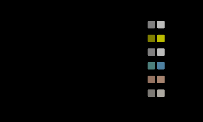
The same blend, taken on the stored values and on the light. Six pairs blended at 50 per cent, once by averaging the values as they are stored and once by averaging the light they stand for. Every resize, every antialiased edge and every transparency composite in an ordinary pipeline does the first. The two land 15.8 colour differences apart at the mean and 19.3 on a red against a green, and the stored-value blend is the darker on all six, by up to 23 units of lightness.

An average on the stored values

A resize, an antialiased edge, a transparency composite and a chroma subsample are all averages, and in almost every pipeline they are taken on the numbers as stored. The numbers as stored are encoded, the encoding is a compression, and a half-and-half blend of black and white taken that way lands 18.7 colour differences from the half-and-half blend of the light — 22.7 units of lightness darker, on every pair, always in the same direction.

applied · Delivery

Named alongside it

The objects these essays reach for when they reach for this one.

Chromatic adaptationConvergenceMeasurement errorSpatial frequencyTest setAliasingResidualDegrees of freedomWavelength gridColour differenceContrast sensitivityDeclared input

All concepts