The matches do not name the cones

A colour match is the only measurement colour science has that is not a matter of judgement. Two lights are put side by side, three knobs are turned until the join disappears, and the numbers are written down. Everything downstream — the standard observer, XYZ, every gamut, every tolerance — rests on that experiment and on nothing softer.

It is also the experiment that cannot tell what the cones are.

The claim #

A colour match is an equality between two triples of integrals. Multiply both sides by any nonsingular 3×3 and the equality survives untouched, so matching data determine the observer’s three curves only up to nine free numbers. What fixes those nine is a different experiment altogether, and this collection has been quoting a matrix that was never fitted to it.

• Nine numbers, exactly. The set of admissible descriptions is the general linear group in three dimensions, which is nine-dimensional. Nothing about the matching data narrows it at all.
• The invariance is exact. Across sixty-four random changes of basis the largest relative discrepancy between a metameric pair’s coordinates is 2.8 × 10⁻¹⁵, which is machine zero rather than a small residual.
• What fixes the nine is dichromacy. Three confusion points, one per class of dichromat, carry six numbers, and three choices of unit carry the rest. Six plus three is nine, and the count is checked here as a rank rather than counted on fingers.
• The matrix this site uses fails that test. Hunt–Pointer–Estévez implies a protanope confusion point 0.13 away in chromaticity from the measured one and a deuteranope’s 1.28 away.
• And that is not a curiosity. Every colour-vision-deficiency figure on this site projects along those directions. Under the matrix built from the measured points instead, the same palette moves by up to 3.9 ΔE00, and across the whole sRGB cube by 1.8 on average and 14.8 at worst.

Why a match cannot see it #

The colour-matching functions are three numbers per stimulus: the integral of the light against each of x̄, ȳ and z̄. Two spectra S₁ and S₂ match for an observer exactly when

∫ S₁ x̄ = ∫ S₂ x̄ and ∫ S₁ ȳ = ∫ S₂ ȳ and ∫ S₁ z̄ = ∫ S₂ z̄

Now replace the three functions with three linear combinations of themselves — x̄′ = a₁x̄ + a₂ȳ + a₃z̄, and likewise for the other two. The new integrals are the same linear combinations of the old ones, and a linear combination of three equalities is an equality. Nothing has been assumed about the combination except that it is invertible, which is required only so that the new triple is still a complete description rather than a projection of one.

So the whole content of the matching experiment is a three-dimensional subspace of the space of functions of wavelength. Which three functions are used to name points in that subspace is free.

The point is easy to under-state, because a reader who has met metameric black already knows that matching throws away most of a spectrum. That loss is a rank argument — three numbers from eighty-one — and it is not this one. This is the loss inside the three: even the three-dimensional summary is only defined up to a change of coordinates, and the change of coordinates is nine parameters wide.

The two losses are worth holding apart, because only one of them is ever taught. The first is the reason two different spectra can be one colour, and every account of colorimetry states it in the first chapter. The second is the reason two different sets of curves can be one observer, and it tends to be mentioned in a footnote if at all — partly because the standard functions are printed so often that they acquire the authority of a photograph, and partly because the alternative descriptions are not usually drawn. Putting one on a handle is the cheapest possible remedy: watching the curves change while the numbers underneath them do not is the argument.

What actually moves #

If the matching predictions do not change, something must, or the freedom would be invisible and harmless.

What changes is every statement about the curves themselves. Where the peaks are, whether they go negative, how wide they are, which one carries the luminance — all of these are properties of the chosen triple and not of the observer.

This matters because the three curves acquire a name at a certain point in the argument. Called colour-matching functions, they are a bookkeeping device and their arbitrariness is obvious. Called cone fundamentals, they are a claim about photoreceptors — that these three curves are, up to a scale, the spectral sensitivities of the three cone classes.

The claim in the second name is not contained in the matching data. It is an additional empirical claim — that the receptor sensitivities lie in the space the matches span — and it is a substantive one, which nothing about colour matching establishes. What colour matching gives, once that claim is granted, is the subspace. Which point of the nine-dimensional family of bases is the receptors’ own is a further question with a further answer.

What fixes them #

The further answer comes from people with two cone classes rather than three.

A protanope has no long-wave cone, so two stimuli look identical whenever they differ only in what that class would have reported. In a chromaticity diagram the confused stimuli lie along a line; the lines for different starting colours are not parallel; and they all pass through one point — the direction the missing receptor would have measured. That point is a measurement, and there are three of them.

Each point supplies two numbers. Three points supply six. The remaining three are the scale of each row, which is a choice of units — here, that the adopting white comes out as one in all three channels. Six plus three is nine, and nine is the dimension of the freedom. The construction is the subject of the next essay; what matters here is that the count comes out exactly, with nothing left over and nothing double-counted.

The path between the two bases is continuous, so a quarter of the way along it is as legitimate a set of fundamentals as either end.

What this collection had been doing #

The machinery behind this site’s colour-vision figures has carried a comment since its first commit saying that a cone-fundamental matrix is a modelling choice rather than a measurement, and naming three that are in use. Years of essays were written on top of that comment. None of them asked what the choice was worth.

The matrix in use here is Hunt–Pointer–Estévez, which is the classic and is what the Brettel–Viénot–Mollon simulation assumes. It was constructed so that a von Kries gain in its axes behaves sensibly under a change of illumination — a good reason for a matrix to exist and an unrelated one. Run backwards through the construction above, it commits itself to three confusion points, and two of the three are in the wrong place.

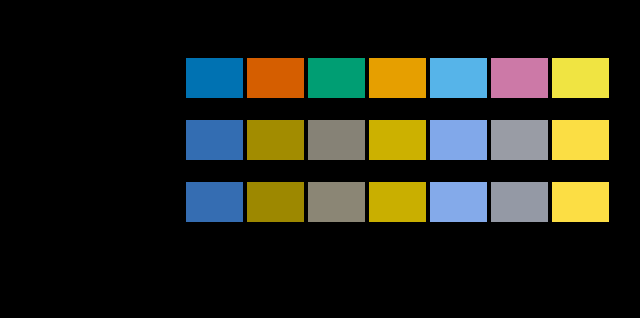
What survives the change is the verdict the site’s own gate asserts — that no pair of the palette collides under any of the three deficiencies. The closest pair under deuteranopia is 11.1 units apart with one matrix and 11.8 with the other, both far clear of the floor. What does not survive is which pair is closest. Under protanopia it is sky blue against reddish purple with one matrix and blue against reddish purple with the other.

That distinction is worth naming, because it recurs. The essay that priced a whiteness figure found the same shape in measurement conditions, where a ranking reversed between two instruments that were both in calibration: a conclusion can be robust to a choice while the evidence offered for it is not. A gate that asserts the conclusion is doing its job. A caption that names the worst pair is quoting the matrix.

What was computed, and how #

The invariance is checked by construction rather than by search. Sixty-four random 3×3 matrices with determinant clear of zero are applied to the tristimulus values of a metameric pair built by this site’s own machinery, and the largest relative difference between the two transformed triples is recorded. It is 2.8 × 10⁻¹⁵. The number is reported rather than merely asserted because an exact statement is best drawn as a residual with its exponent visible.

The count is checked as a rank. The nine inputs — two coordinates for each confusion point and one scale per row — are perturbed one at a time, the nine matrix entries are differenced, and the singular values of the resulting 9 × 9 Jacobian are taken. All nine are well clear of zero, with a condition number of about twenty-one. Had two inputs moved the matrix the same way, or one moved it not at all, a singular value would have collapsed and “six plus three is nine” would have been arithmetic hiding a degeneracy.

The construction is checked against the literature rather than against itself. Running impliedCopunctal on the Smith–Pokorny fundamentals — which are the standard set derived from the confusion points — returns those points to within 1.9 × 10⁻⁴, which is the rounding in the published matrix. That is the only available evidence that the algebra here is the algebra the field uses rather than a plausible rearrangement of it.

The simulation gap is the Brettel–Viénot–Mollon projection run twice with the cone matrix as an argument, compared in ΔE00 in CIELAB. The construction is repeated here rather than parameterised in place because the shipped simulator memoises its projection planes against the matrix it was built with, and a parameter no essay would ever pass is a worse thing to add than three lines of duplication.

What the invariance amounts to is best seen on a single matching pair, scored somewhere in the middle of the path rather than at either end of it.

Where the model stops #

The confusion points are themselves measurements and carry their own uncertainty. They come from far fewer observers than the matching functions do, and tritanopes are rare enough that the short-wave point is the least well determined of the three. So the nine numbers are not known to the precision the arithmetic here implies; they are known to the precision of a smaller experiment. That is a real weakness of the repair and it does not restore the matching data’s ability to choose.

The Brettel construction is a model of dichromacy and not a report from one. Nothing above says what a dichromat sees. What is measured is the difference between two simulations, which is a statement about this site’s machinery.

And the freedom is nine-dimensional only if the observer is exactly three-dimensional. Rod intrusion, a fourth photopigment class in some observers, and any departure from the additivity laws would change the shape of the argument rather than its size. Within the band where matching is trichromatic and additive, which is where all of colorimetry lives, the count is exact.

Who found it, and when #

The structure is König’s. Arthur König and Conrad Dieterici’s work in the 1880s and 1890s took the dichromat confusion data and used them to pull cone sensitivities out of matching functions, and the construction has carried his name ever since. Maxwell had already established in the 1850s that colour matching is three-dimensional and linear, which is the premise; the step König added is that a second population, missing one receptor, supplies exactly the constraints the first population cannot.

The modern versions are Smith and Pokorny’s from 1975 and Stockman and Sharpe’s from 2000, and the second is what the CIE’s physiological observer is built on. Both are constructions in this sense: matching data plus something else. The something else is usually mentioned once, in a methods section, and then the resulting curves are printed as though they were measured directly.

Hunt–Pointer–Estévez arrives from a quite separate tradition. It belongs to the appearance-modelling literature, where the requirement on a set of axes is that scaling them independently should reproduce what happens to appearance when the light changes — the von Kries hypothesis with a basis attached. A matrix chosen to make that work has every right to exist and no obligation to land on the receptors, and its own literature does not claim that it does. The claim gets added later, by everybody who reads the letters L, M and S at the ends of its rows.

The cost of the freedom is not in what the matches say but in what the diagram looks like, and halfway along the path is where that is easiest to price.

The generalisation #

The pattern is a model whose parameters split into three kinds, of which only the first is ever reported: the ones the data determine, the ones the data leave on an orbit, and the ones fixed by a convention nobody records.

The diagnostic is cheap and almost nobody runs it. Take the transformation group under which the data are invariant, apply it, and see which of the published claims change. Anything that changes was a statement about the convention. A fit reported with a residual and no orbit is half a result, and the missing half is not an error bar — an error bar is about noise, and this is about a direction in which the data say nothing at all.

The condition number is a caveat, not a reassurance #

The rank check is reported as evidence that the construction is a bijection — nine singular values clear of zero, “with a condition number of about twenty-one”. The first half is what the check was for and it passes. The second half is a measurement the essay quotes and does not read.

A condition number of 21 says the worst-determined direction of the nine-parameter map is twenty-one times less well determined than the best. A one per cent uncertainty in the inputs can arrive as a twenty-one per cent uncertainty in some combination of the matrix entries, and the smallest singular value is a twentieth of the largest.

That lands directly on the weakness the essay already declares. The confusion points are measured on far fewer observers than the matching functions, and the short-wave point is the least well determined of the three, because tritanopes are rare. So the repair takes the least reliable of its three inputs and passes it through a map that can amplify a relative error twentyfold along one direction. Which direction that is has not been asked, and it is answerable with the singular vectors the check already computes: if the worst-conditioned direction is the one the tritan point moves along, the repair is much softer than its arithmetic suggests; if it is a direction the protan point controls, the repair is on firm ground.

Twenty-one is not a bad condition number for a nine-parameter geometric construction, and nothing here says the matrix is wrong. It says the check answered is the map invertible and printed, in passing, the answer to how well — and the second answer belongs beside the first weakness in the list, not in the sentence establishing that the count comes out.

Two gaps on a scale that does not carry them #

The protanope point implied by Hunt–Pointer–Estévez is 0.13 from the measured one and the deuteranope’s is 1.28 — quoted together, a ratio of ten to one, and read as a statement that one of the two is far worse.

It may be, and these two numbers do not establish it. A chromaticity distance is a common unit and the three confusion points do not sit at comparable places: a copunctal point lies wherever the pencil of confusion lines happens to converge, which for two of the three classes is well outside the spectral locus and for one is a long way outside it. What the simulation actually depends on is the direction of the lines through the point, not the point’s position, and the map from one to the other depends on how far the point sits from the region being simulated. A displacement of 1.28 at a point far away and a displacement of 0.13 at a point nearby need not be in the ratio their numbers are in.

The essay never makes that conversion, and neither of the two figures it does report — the palette’s 3.9 ΔE00 and the cube’s 14.8 — is broken out by deficiency, so nothing on the page says whether the larger positional gap produces the larger simulation error. That is the missing column, it costs nothing to compute from the machinery already in place, and until it exists the two gaps should be read as both nonzero rather than as one ten times the other.

What the palette misses #

Two of the reported numbers are measurements of the same thing over different sets, and comparing them says something about the set this collection checks its own figures against.

Over the palette, the worst colour moves 3.9 ΔE00 between the two matrices. Over the whole sRGB cube, the mean is 1.8 and the worst is 14.8 — nearly four times the palette’s worst, and eight times the cube’s own mean.

So the palette is not unrepresentative on average; its worst case is comfortably above the cube’s mean. What it misses is the tail, and it misses it by a factor of four. That is not an accident of sampling: the palette is a set of colours chosen to stay distinguishable under all three deficiencies, which means it was built to avoid exactly the regions where a dichromatic projection is most sensitive to its axes. A set selected for robustness will under-report the cost of a change of basis, and the site’s own gate runs on that set.

And the verdict is far steadier than the evidence #

The last comparison is the one the essay names and does not size. Individual palette colours move by up to 3.9 units between matrices; the closest pair under deuteranopia moves from 11.1 to 11.8, which is 0.7 units — 18 per cent of the largest single-colour displacement.

That ratio is the mechanism behind the essay’s own observation that a conclusion can be robust while its evidence is not. A change of basis is a smooth map, so two nearby colours are displaced in nearly the same direction and by nearly the same amount, and their separation is the part of the displacement that does not cancel. Positions move by a lot and distances between them move by a little, which is why a gate asserting a minimum separation survives a choice that moves every number it is computed from.

Where the ladder goes next #

The freedom acts on a chromaticity diagram as a projective map, which preserves straight lines and preserves neither area nor angle. So every claim about a shape on the diagram inherits the choice, including the one this collection has made most often — that about two thirds of the visible diagram cannot be shown on a screen.

And the freedom stops being free the moment a nonlinearity is applied. CIELAB divides by a white point and takes a cube root, and a cube root does not commute with a change of basis — so every colour difference on this site is computed downstream of a choice that was made without colour difference in mind.