No diagram makes them circles
Assumes MacAdam measured it, The diagram was replaced in 1976 and The diagram has no area.
MacAdam’s ellipses are the most quoted embarrassment in colour science. Twenty-five contours of just-noticeable difference, measured on one observer in 1942, drawn on the CIE diagram at ten times actual size because at true scale most of them are thinner than a line — and varying by an order of magnitude in size and by a factor of several in shape across the picture.
The standard reading is that the 1931 diagram is a bad ruler. That is true. The question nobody puts a number on is how much of the badness belongs to the diagram.

The claim
A change of coordinates in the observer acts on the diagram as a projective map, so the ellipses’ failure to be circles can be minimised over the entire nine-parameter freedom. It can be reduced and it cannot be removed: the best plane leaves a mean axis ratio of 2.02, which is therefore invariant and is a property of the measurement rather than of the picture.
- CIE xy gives a mean axis ratio of 2.95 and a size spread of 10.42.
- The 1976 u′v′ revision gives 2.37 and 2.21.
- The best plane found by search gives 2.02 on shape, or 1.79 on size, and nothing does better on either.
- So the revision took 95 per cent of the available improvement in size and 62 per cent of it in shape, which is a much more interesting verdict on 1976 than “it is more uniform”.
- And the residual 2.02 is invariant, in the exact sense that no member of the nine-parameter family beats it. Anisotropy of about two is what the eye does.
What is being minimised
Two numbers, both ratios, and both are the pair this collection uses to rank spaces — measured here on a two-dimensional plane rather than in a three-dimensional space.
Anisotropy is the mean over the twenty-five of the longest radius divided by the shortest. It asks whether a step of a given size means the same thing in every direction. One would mean every contour is a circle.
Spread is the largest mean radius divided by the smallest, across the set. It asks whether a step of a given size means the same thing everywhere on the diagram. One would mean every contour is the same size.
They are different failures and a diagram can trade one for the other, which turns out to be exactly what happened in 1976.

The search
The freedom is the nine coefficients of a nonsingular matrix applied to the observer’s three functions, of which an overall scale cancels in a chromaticity — so eight parameters act on the plane. Each ellipse’s measured boundary is carried through: the boundary points are converted to tristimulus values at a fixed luminance, mapped, divided through, and the radii from the transformed centre are measured.
The boundary points are mapped rather than the quadratic form, and the reason is that a projective map is only locally affine. Transforming a conic exactly would need the map’s Jacobian at each centre, which is an approximation at the scale of the ellipse; mapping the measured points is exact at every point and costs nothing.
The optimiser is a restarted Nelder–Mead over the nine coefficients. Three of the nine do nothing at all, since the overall scale cancels, and the search is left to discover that rather than being told — a parametrisation that removed them would have to choose which three, and the choice is arbitrary. What it costs is a flat direction in the cost surface, which is precisely the situation a plain simplex reports a false convergence in and a restarted one does not.


The floor, and why it is the finding
An optimum that is not reached is a statement about an optimiser. An optimum that is reached and is still bad is a statement about the problem.
The search converges from many restarts to a mean axis ratio of about 2.02, and no configuration tried beats it. That number is therefore a property of the twenty-five measured ellipses and of nothing else — it survives the entire freedom that colour matching leaves in the observer, in exactly the sense that collinearity survives it and area does not.
The interpretation is the one the ellipses were always taken to support and could not, until now, be shown to support. Discrimination is anisotropic in a way that no linear redescription of the observer can absorb. The failure is not that somebody picked awkward primaries in 1931.


What an anisotropy of two means
Two is a number worth converting into something a reader can picture, because “the ellipses are not circles” is a statement everybody accepts and nobody has to act on.
An axis ratio of two means that at the average place on the diagram, a step in the worst direction is twice as detectable as a step of the same size in the best direction. A tolerance drawn as a circle around a target therefore accepts twice as much error along one axis as along the other, and which axis depends on where the target sits. That is not a small correction: it is the difference between a pass and a fail on a substantial fraction of any real production run, and it is why a tolerance has to be a shape rather than a radius.
It also sets a limit on what a scalar difference formula can be asked to do. A single number cannot encode a direction, so any formula reporting one has to average over directions somewhere, and the averaging is worth a factor of two at the point where it happens. Every parametric factor in a modern difference formula is a way of moving that averaging around rather than removing it.
The size spread is a different and in some ways worse failure. A floor of 1.79 means the best available diagram still has one region where a just-noticeable step is nearly twice as long as in another — so a fixed tolerance is nearly twice as strict in one part of colour space as in another, before any question of direction arises.
What the 1976 revision actually did
The CIE’s 1976 diagram is u′ = 4X / (X + 15Y + 3Z) and v′ = 9Y / (X + 15Y + 3Z), which is a projective map of the 1931 coordinates and is therefore one member of the family searched here. Setting it against the floor turns a qualitative verdict into two numbers.
On size spread it took 8.21 units of the 8.63 available — 95 per cent. That is close to everything there was, and it is why the revision is remembered as a success.
On axis ratio it took 0.57 of the 0.93 available — 62 per cent. That is a real improvement and it leaves a third of the achievable gain on the table, on a failure whose floor is high anyway.
Two caveats on the credit, and one of them matters
The two percentages are the sharpest thing in this essay and both need a line of qualification before they are quoted anywhere.
The credit is a linear difference between two ratios, and a ratio’s natural scale is logarithmic. An anisotropy of four is to two what two is to one; a difference of 8.63 between a size spread of 10.42 and one of 1.79 is dominated almost entirely by the top of that range. Recomputing both credits in logarithms:
On size the revision took 88 per cent of what was available, not 95. On shape it took 58 rather than 62. Neither reading is wrong and the difference between them is not decoration: seven percentage points is the gap between almost everything there was and most of it, and the first is the sentence that would be repeated.
The shape figure barely moves, because 2.95 and 2.02 are close enough together that linear and logarithmic distances nearly agree. The size figure moves because 10.42 and 1.79 are not. Whenever a credit is computed between two ratios that differ by an order of magnitude, the scale it is computed on is part of the answer, and the honest form quotes both or says which.
And the two floors are two different diagrams
The other caveat is structural and it is the one the “or” in the claim is carrying.
The best plane for shape gives 2.02. The best plane for size gives 1.79. They are not the same plane. No single chromaticity diagram achieves both floors, so the two credits are scored against two ideals that cannot be met at once, and adding them or averaging them would mean nothing.
The published diagrams make the trade visible without any search at all. The 1960 u v diagram sits at 2.19 on shape and 2.35 on size; the 1976 u′v′ at 2.37 and 2.21. The 1960 diagram is eight per cent better on shape and six per cent worse on size, so neither dominates, and the 1976 revision was not an improvement in the sense of being better at everything — it was a step along a front, in the direction of size.
That reframes the verdict the credits are meant to deliver. Read as two independent scores, the revision looks like a near-complete success on one axis and a partial one on the other, and the natural question is why the second axis was left half-done. Read as one point on a trade-off, it looks like a deliberate choice of where to sit — and the 1960 diagram sitting on the other side of the same front is the evidence that the choice was available and was made.
Which means the remaining forty per cent on shape may not be available at all, at this size spread. The floor of 2.02 is what the best shape plane achieves, and that plane’s size spread is not reported here; if it is worse than 2.21, then a diagram taking the rest of the shape improvement would be giving back some of the size improvement, and the revision would have been trading rather than leaving something on the table.
Establishing that needs one more computation and it is the natural completion of this essay: sweep the constraint rather than optimising each criterion alone, minimising anisotropy subject to a size spread no worse than a stated value, and draw the front. Both published diagrams would then sit on it or inside it, the two floors would be its two ends, and the question of whether 1976 left anything on the table would have an answer instead of an implication.
The 1960 u v diagram it replaced does better on shape (2.19) and worse on size (2.35). Neither diagram dominates the other, which is the ordinary situation when two criteria are traded and one is chosen, and it is why the change was not universally welcomed at the time.
What was computed, and how
The ellipse data are MacAdam’s published semi-axes and orientations and are quoted rather than computed, on this collection’s rule that a measurement of people is quoted and everything downstream of it is not.
Each ellipse is sampled at sixty-four boundary points at true scale. The radii are measured in the transformed plane from the transformed centre; the anisotropy is the mean over ellipses of max over min; the spread is the ratio of the largest mean radius to the smallest. Both are dimensionless, which matters because the twelve planes have wildly different natural magnitudes and a raw distance would report nothing but that.
The luminance the chromaticities are realised at is a stated choice and is 0.4. It has to be chosen — a chromaticity carries no luminance of its own — and the projective action does not depend on it, so it affects nothing here. Any figure quoting these numbers says which value it used.
The assertion is set at a floor of 1.8 rather than at the measured 2.02, on the standing rule that an assertion set at exactly what was measured fails the next time anything changes. It is accompanied by a second assertion that the search beats the default diagram, because a floor on its own would also pass if the optimiser did nothing.
Where the model stops
Twenty-five ellipses, one observer, 1942. MacAdam’s data are a measurement of one person’s discrimination at one luminance, and everything in this essay inherits that. A modern replication with more observers would move the floor; there is no reason to think it would move it to one.
The ellipses are chromaticity contours and discrimination is three-dimensional. A step in lightness is not represented at all, so this is a statement about the plane rather than about colour difference in full. The three-dimensional version is what a ΔE formula computes, and it is computed after a nonlinearity, which changes the problem entirely.
The two summary numbers are means and maxima and hide their own distributions. A mean axis ratio of 2.02 is consistent with most ellipses being nearly round and a few being very elongated, which would be a different situation from all of them being moderately elongated, and the summary does not say which. The per-ellipse values are computed and available to the figures; what is asserted is the mean, because that is the quantity the optimisation minimises and asserting something the search did not optimise would be asserting an accident.
And a projective map is the whole of the freedom only because the observer’s freedom is linear. Nothing here bears on the much larger question of what a nonlinear redescription could do — and the answer to that is not in doubt: CIELAB, CIELUV and Oklab are all nonlinear and all do better than any chromaticity plane. That is not a rival result; it is a different problem, and it comes with a basis choice of its own.
Who found it, and when
MacAdam published the ellipses in 1942 and immediately understood what they implied about the diagram; the search for a better projective picture began at once and produced Judd’s 1935 attempt, the CIE’s 1960 adoption of MacAdam’s own u v diagram, and the 1976 revision.
What appears not to have been done, or at least not to have become standard knowledge, is the optimisation over the whole family. The literature contains a sequence of proposals, each better than the last, and the natural question — how much room is left — is answered by a search that costs a second on a modern machine and could not be run in 1960.
The conclusion is not a criticism of the people who made the proposals. It is the difference between an era in which one evaluates candidate diagrams and one in which one can characterise the whole space of them, and it is a difference in instruments rather than in insight.
The generalisation
The shape is a defect attributed to a convention, where the convention turns out to be responsible for part of it and the measurement for the rest, and nobody had separated the two.
The separation is available whenever a group acts on the representation: minimise the defect over the group, and whatever is left is the measurement’s. It is a cheap and general move and it converts an argument about which convention is best into two numbers — how much the current one loses, and how much is there to lose.
The failure mode it prevents is the long-running search for a better convention when the floor is close. Sixty per cent of the available improvement in shape was taken in 1976, and a reader who did not know the floor could reasonably conclude that another revision might take the remaining forty and reach uniformity. It would not.
The same move is what the observer’s own freedom demanded and it is worth noticing that the two run in opposite directions. There the group was applied to find out what the data cannot determine, and the answer was a warning. Here it is applied to find out what a convention cannot be blamed for, and the answer is a floor. Both are the same operation — quotient by the group and see what is left — and it is the residue that carries the information in each case.
Where the ladder goes next
The nonlinear spaces do better and they pay for it: a cube root does not commute with a change of basis, so a lightness-chroma space is a property of the basis it was built on as well as of the observer — and CIELAB’s basis was chosen in 1931 for reasons that had nothing to do with colour difference.
The other direction is what a floor like this one is worth to a practitioner. A tolerance is a shape precisely because the contours are not circles, and an anisotropy of two is the number that makes a box in a colour space the wrong container.
Where this goes next
 MacAdam measured it
In a perceptually uniform space the just-noticeable-difference contours would be circles of equal size. MacAdam's ellipses are neither, by a factor of eighty — and transforming them into each candidate space settles which spaces improved matters and by how much.
MacAdam measured it
In a perceptually uniform space the just-noticeable-difference contours would be circles of equal size. MacAdam's ellipses are neither, by a factor of eighty — and transforming them into each candidate space settles which spaces improved matters and by how much.
 The diagram was replaced in 1976
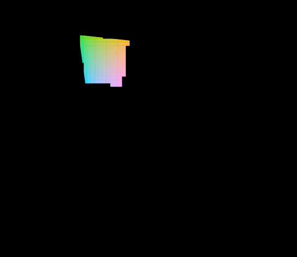
The CIE knew the 1931 diagram was badly distorted and published a better one. Half a century later almost every chromaticity plot in print is still the old one, and both are still printed filled edge to edge with colours no display can show.
The diagram was replaced in 1976
The CIE knew the 1931 diagram was badly distorted and published a better one. Half a century later almost every chromaticity plot in print is still the old one, and both are still printed filled edge to edge with colours no display can show.
 The diagram has no area
A chromaticity diagram is a projective picture of a three-dimensional space, and the freedom colour matching leaves in the observer acts on it as a projective map. Straight lines and mixture ratios survive that; area, distance and angle do not — so half of what the diagram is used to say is a statement about the paper.
The diagram has no area
A chromaticity diagram is a projective picture of a three-dimensional space, and the freedom colour matching leaves in the observer acts on it as a projective map. Straight lines and mixture ratios survive that; area, distance and angle do not — so half of what the diagram is used to say is a statement about the paper.
What this makes readable
Essays that name this one as a prerequisite.
Named alongside this one
Essays reaching for the same objects. Nobody chose these; they are what the index of named objects makes visible.
- A compression goes below the floor chromaticity plane · cielab · identifiability · invariance · macadam's ellipses · perceptual uniformity · projective transformation
- How many colours are there cielab · δe · just-noticeable difference · macadam's ellipses · perceptual uniformity
- Where the formula is not smooth cielab · δe · just-noticeable difference · macadam's ellipses · perceptual uniformity
- Which of two is worse cielab · δe · just-noticeable difference · macadam's ellipses · perceptual uniformity
- A threshold is not a unit δe · just-noticeable difference · macadam's ellipses · psychophysics
- The exponent was never the argument cielab · identifiability · macadam's ellipses · perceptual uniformity
What links here
The 8 essays that link to this one and share the most of its objects, of 16 that link here.
The objects this essay names
Each one links to every other essay that touches it.
Chromaticity planeCIELABΔEIdentifiabilityInvarianceJust-noticeable differenceMacAdam's ellipsesPerceptual uniformityProjective transformationPsychophysicsUniform chromaticity scale