A scene has no white point

The algorithms that guess the light treats illuminant estimation as an underdetermined problem to be attacked with assumptions, and measures how badly each assumption fails on a scene built to violate it. Grey-world reaches 43.1° of angular error on an all-green scene; no estimator wins everywhere; a camera choosing one has chosen which photographs to be wrong about.

All of that assumes the question has an answer. Often it does not.

The claim #

White balance applies one transform to a whole image. A scene lit by two lamps needs a different transform at every point, and no choice of the single transform is correct anywhere except where it was chosen.

This is not a statement that estimation is difficult. It is a statement that the thing being estimated does not exist as a single quantity, so improving the estimator cannot help.

What the computation shows #

Take one neutral surface — flat reflectance, no colour of its own — and light it with mixtures running from illuminant A at one end to D65 at the other. That is an ordinary domestic scene: a room with a tungsten lamp and a window.

Every patch is the same object. The only thing varying across the sequence is how much of each lamp reaches it, which depends on where it is standing.

Now apply one diagonal correction, chosen so that the middle of the run comes out neutral. The generator asserts both halves of the result: the middle patch is neutral to well under a unit of $\Delta E_{00}$, and both ends are more than three units away from neutral.

A single transform is exact at one point and wrong everywhere else, and the error grows with distance from where it was chosen. No estimator produces a better single number, because the residual is not estimation error. It is the scene’s own variation, and it survives any choice.

Why this is different from ordinary estimation error #

The distinction is worth labouring because the two failures look identical in an image and have completely different remedies.

Estimation error is a wrong answer to a well-posed question. The scene has one illuminant, the algorithm guessed badly, and a better algorithm would do better. The residual is uniform across the image — everything is too warm, or everything is too green — and a single correction fixes it.

Under-specification is a well-executed answer to a question with no single answer. The residual varies across the image, and no single correction fixes it, because the thing to be corrected is different in different places.

The diagnostic is the spatial structure of the residual. A uniform cast is an estimation failure; a cast that changes across the frame is not. That is why the shadows in a photograph are the part that has to be graded by hand, and why the difficulty concentrates at boundaries between lit regions rather than being spread evenly.

The two-lamp scene is the normal case #

It would be reasonable to treat all this as an edge case if mixed illumination were rare. It is close to universal.

Outdoors there are always two. The direct beam and the sky are different spectra by construction, differing by 21.4 units of $\Delta E_{00}$ between their whites, and every surface sees a different mixture depending on how much sky it can see. A scene with any shadow in it is a two-illuminant scene.

Indoors during the day there are always two. A window and a lamp, and their mixture varies with distance from the window.

In a room with one lamp there are still several. Five of six surfaces emit nothing and are lit entirely by interreflection, so the effective illuminant at a point is the lamp multiplied by whatever it bounced off — a different spectrum for each surface, set by the form factors.

So the single-illuminant scene is the special case: one source, no windows, neutral surroundings, nothing bouncing. That is a light booth, and light booths are built that way deliberately, painted neutral grey rather than white for exactly this reason.

How large is the residual #

The size of the unfixable part is worth quantifying, because “no single answer” is only interesting if the spread is big enough to matter.

Between illuminant A and D65 the two whites differ by a great deal — A is a Planckian radiator at 2856 K and D65 is daylight — so the run above is close to a worst case for an interior. At the ends the residual after correction exceeds three units of $\Delta E_{00}$ in the figures, against a tolerance for a coating of under one.

Outdoors the spread is comparable and arrives for a different reason. Open ground and shadowed ground sit under illuminants 21.4 units apart, and unlike the indoor case there is no arrangement of the scene that avoids it — the sky and the sun are both always present, and the mixture is set by geometry the photographer does not control.

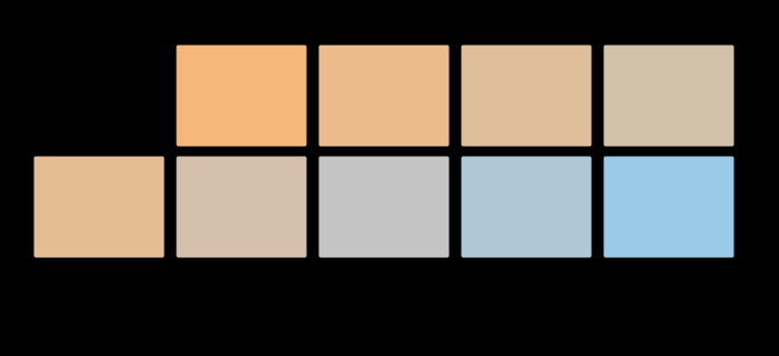
How many steps the mixture is sampled at is a drawing choice; how far apart the two lamps are is not.

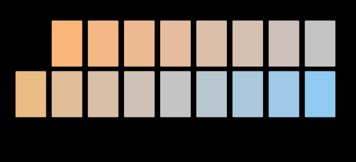
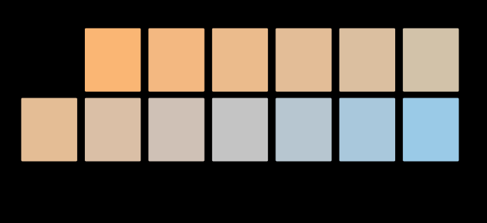
So the honest summary is that the residual scales with how far apart the illuminants are, is zero only when they coincide, and reaches several times a commercial tolerance in ordinary domestic and outdoor scenes. It is not a corner case and it is not usually the largest error in a photograph; it is the one that cannot be reduced by trying harder at the step that produced it.

What the residual actually is, and where it is worst #

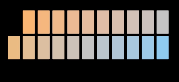
The assertion demands more than three units at each end, which is a floor rather than a reading. With the correction set at the middle of an A-to-D65 run, the tungsten end is left at 19.80 ΔE00 and the daylight end at 16.90, against a coating tolerance of one, and the mean across the whole run is 10.76.

The asymmetry between the two ends is the smaller of the two surprises. The warm end is worse by nearly three units, because reaching it takes a large blue gain and the space the difference is measured in is not symmetric about the target white.

The larger surprise is the shape. The residual does not grow in proportion to how far a patch sits from where the balance was chosen; it grows fastest right beside it. A patch a tenth of the way along the mixture is already at 5.48, and one two tenths along is at 9.98 — half the total error, a fifth of the way across the scene. The increments then fall away steadily: 5.48, 4.50, 3.78, 3.23 and 2.81 for each further tenth.

So being near the reference is worth much less than it sounds. The stretch a single white balance genuinely serves is far narrower than the run it was chosen from, and “the error grows with distance” understates how quickly the growing is finished.

What the best possible single choice buys #

If this were a badly chosen white point, choosing it well would help, and how much it would help can be worked out exactly rather than argued about.

Sweeping the reference across the whole mixture in hundredths and scoring each choice over the entire run: the mean residual is lowest at a mixture of 0.57 rather than at the midpoint, and it is lowest at 10.656 against the midpoint’s 10.760. That is one tenth of a unit, on a residual of eleven. Choosing instead to minimise the worst patch moves the reference to 0.43 and improves the worst case from 19.80 to 18.69, a saving of 1.11 units, or six per cent.

That is the essay’s claim in the form a sceptic would ask for. The failure is not a mis-set parameter, because setting the parameter optimally recovers one per cent of the mean error and six per cent of the worst. Any estimator, however good, is competing for the tenth of a unit between the obvious choice and the best one — and the eleven units underneath it belong to the scene.

Sampling the run more finely says whether the failure at the ends is a property of the two lamps or of how coarsely the mixture was walked.

How it scales with the two lamps #

The residual is worse than proportional to how far apart the lamps are, which “scales with” leaves open.

Tungsten against D65: the two whites are 26.76 ΔE00 apart and a single correction leaves 19.80 at worst, which is 74 per cent of the separation. Tungsten against D50: 24.52 apart, 16.99 left, 69 per cent. D50 against D65: 12.82 apart, 6.62 left, 52 per cent.

So bringing two lamps closer together does more than reduce the residual in proportion. It reduces the share of their difference that a single transform fails to remove, from about three quarters to about half. Matching the lamps in a room is therefore worth more than the distance between their chromaticities suggests — which is the practical advice this argument implies and which the argument nowhere states.

Why the correction is diagonal, and why that is a second problem #

There is a separate approximation buried in “one transform” that is worth separating from the main claim.

A white-balance correction is almost always diagonal: three independent gains, one per channel. That is von Kries adaptation, it is one of the four ways to move a white point on this site, and it is exact only if the sensor’s channels happen to be the right basis.

They are not, and the better chromatic adaptation transforms — Bradford, CAT16 — first rotate into a sharpened cone-like space, apply diagonal gains there, and rotate back. The improvement is real and it is a refinement of the same operation.

None of it addresses this page’s problem. A better adaptation transform gives a better single answer; the objection here is to there being one. Improving the transform and applying the wrong number of them are independent failures, and the literature is much richer on the first.

What was computed, and how #

The mixtures are spectral. Each patch is the sum of two illuminant spectra in stated proportion, multiplied by a flat reflectance, then integrated — not an interpolation between two RGB values, which would have assumed the answer.

The correction is a diagonal transform in XYZ, computed as the ratio between the target white and the white of the mixture at the chosen reference point. That is the simplest von Kries-type correction and it makes the argument without a choice of cone space complicating it.

The white point is normalised before the comparison, and getting that wrong hid the whole effect once. The first version compared a patch at $Y = 0.5$ against a white point at $Y = 10567$ — which is what integrating an unnormalised spectral power distribution gives. Every ratio landed at $5\times10^{-5}$, deep inside CIELAB’s linear branch, and every patch came out at $L^* = 0.04$ with $a^* = b^* = 0$. The figure reported a perfect white balance across a scene it had just drawn running from $x = 0.399$ to $x = 0.250$. Nothing overflowed, nothing threw, and the only reason it was caught is that the assertion demanded the ends be wrong and they were reported as right.

That is the fourth time this site has been saved by an assertion phrased as “this must fail”, and the pattern is consistent: a check that something is broken catches a collapse that a check that something is fine would have passed.

The mechanism deserves stating in general, because it is not specific to CIELAB. A conversion that expects two quantities on the same scale, given them on different scales, does not error — it lands in whichever part of its domain the ratio implies. For CIELAB that part is the linear branch near zero, where the cube-root is replaced by a line through the origin and all the chromatic information is compressed towards nothing. The function is behaving exactly as specified; the specification assumed a normalisation that the caller had not performed. Anywhere a formula divides one measurement by another, the units and the normalisation are part of the contract and are almost never checked.

What the pictures cannot show #

The real phenomenon is a spatial gradient and a row of patches is not. A photograph of a mixed-lit room shows the cast varying continuously across the frame, and that continuity is what makes it unfixable by a global operation and also what makes it hard to see in a swatch row.

Some corrected patches are outside the display’s gamut, particularly at the tungsten end where the correction applies a large blue gain, and where they are the figures hatch rather than clip — marking rather than approximating.

Nothing here says what the scene looks like. A person standing in a mixed-lit room does not perceive a strong cast, because constancy discounts most of it and because adaptation is at least partly local rather than global. The visual system is not applying one transform to the whole visual field, which is precisely the capability a camera lacks. The gap between what an instrument reports and what a person sees is the whole reason matching and appearance are separate fields here.

Where the model stops #

Two illuminants, one dimension. Real scenes have several sources and a two-dimensional distribution of mixtures. The argument gets stronger, not weaker.

Neutral surfaces only. Every patch here is a grey card, so the mixture is visible directly. With coloured surfaces the illuminant and the reflectance are multiplied together and cannot be separated, which is the underlying difficulty of the whole subject — and the grey card is doing exactly the job a highlight does on a glossy object, supplying a region where the illuminant is present nearly undisturbed.

One correction target. Everything here corrects towards D65. Correcting towards a different white moves all the patches together and changes none of the differences between them, so the choice is presentational; what is not presentational is that there is one target rather than a field of them.

Diagonal correction in XYZ. A sharpened transform would reduce the residual somewhat and cannot remove it.

No spatially varying correction. Local white balance is possible and is what modern computational photography actually does — estimate an illuminant map rather than an illuminant. That is a real answer to this problem and it is outside this model, which computes what the standard single-transform pipeline does.

And no interreflection between the two lit regions. In a real room the tungsten-lit part reflects light onto the daylit part and back, so the mixtures are not independent — each region contributes to the other’s illuminant, which the field’s base rung describes and which this scene does not include. It smooths the gradient and does not remove it.

The generalisation #

The transferable form is about the shape of a specification rather than about colour.

When a model takes a single value for something that varies, the residual carries the variation and gets attributed to noise. The tell is that the residual is structured — correlated with position, time, or whichever variable the model collapsed. Estimation error is unstructured; under-specification is structured, and the two are distinguished by looking at the residual rather than at its magnitude.

The remedy is never a better estimate of the single value. It is either to admit the field is a field, or to state the scope within which the single value applies. Colour management chose neither: a profile has one white point, and there is no place in the format to say the image contained two. So the information that would have diagnosed the problem is discarded at the moment the file is written, and everything downstream inherits an assumption it cannot see.

Who found it, and when #

Von Kries proposed independent scaling of the three receptor responses in 1902, and the coefficient rule that carries his name is still the skeleton of every white-balance operation performed today. He was describing adaptation in the eye rather than an image-processing step, and the eye’s version is not global — which is a difference that took a long time to matter, because for most of the twentieth century nobody was applying the rule to a whole photograph at once.

Land’s retinex work from the late 1950s onwards is the point where the locality became the subject. His demonstrations with mixed illumination are exactly this page’s scene, built physically, and his argument was that the visual system computes ratios locally rather than applying a global correction. Whether retinex is a good model of human vision has been argued about ever since; that it identified the right problem is not in dispute.

The colour-management standards took the opposite path and are worth naming for it. ICC profiles were designed around a device, and a device has one characterisation — which is exactly right for a printer or a monitor and imports an assumption into every image that passes through one. A profile’s white point describes the conditions the device was characterised under; applying it to a photograph silently asserts that the photograph’s scene had one too. The assumption is invisible because it was never stated as an assumption about scenes.

Computational photography arrived at the same place from the other end, and comparatively recently. Illuminant maps rather than illuminant estimates became practical only once there was enough computation per image to support them, and the standard file formats still have nowhere to record one. So a phone may estimate a spatially varying illuminant, apply it, and then write a file whose metadata claims a single white point — which is honest about the output and silent about the operation.

Where the ladder goes next #

The neighbour on this rung is the same problem seen from the instrument’s end: gloss changes the measurement, where one sample returns two different and both-correct numbers depending on the geometry the instrument chose, and where the specification again has no field for the thing that decided the answer.

Below, the field’s base rung is where the multiplicity comes from: a bounce is a multiplication, and a room in which light bounces has as many illuminants as it has surfaces.