A pool with an edge
Assumes What a still eye stops seeing, A fading pool has a shape and Brightness is inferred from edges.
This collection’s model of a stabilised image is a Gaussian pool of local adaptation, and it answers one question well: what survives is everything finer than the pool, so a stabilised disc loses its interior and keeps its outline. It cannot answer the next question, and the reason is structural rather than a matter of tuning. A Gaussian has no edge. A kernel averages across a contour exactly as happily as along it, so the model has nothing to say about what the inside of a faded region actually becomes, nor about why the answer is a region with a shape.
The claim
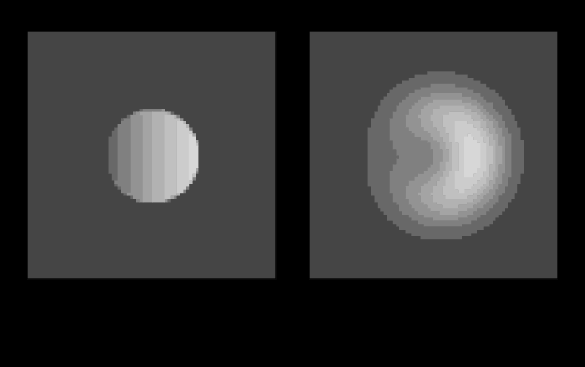
Replace the kernel with a diffusion that contours block, and the steady state inside a closed region is harmonic — so its value at the centre of a disc is exactly the mean of its border. The interior takes the average of its own boundary, not of its neighbourhood, and it does so however the boundary varies.
- Measured: the centre settles to the border mean to within 8 × 10⁻⁹ of the border’s own range, on a 161-square field — a solver tolerance rather than a discretisation error.
- The kernel misses it by 60 per cent of the range, because it weights the near rim more than the far one and a filled region does not.
- The mechanism adds one thing — a permeability that varies with the image — and no free parameter the old model did not have.
- And it reduces to the old model where there are no contours: with an empty boundary map the reach is 0.484°, against a stated pool extent of 0.5°.
What changes, and what does not
The old model is a local pool of Gaussian extent σ that tracks the image blurred by itself; adaptation is complete when the gain cancels that blurred copy, so what is left driving the channel at spatial frequency f after time t is 1 − a(t)·P(f). Everything the fading essays say is that expression read in different directions, and it is a high-pass filter that switches on over a minute.
The new model replaces the kernel with a partial differential equation. The local signal diffuses, and the contours in the image are where it cannot go:
The permeability at each point is one minus the contour strength there, so a contour is a wall. The signal is injected along the surviving edges, and there is a slow leak towards the resting state. Everything below is that equation read in one direction or another.
It adds one mechanism and no free parameter. The pool’s extent σ and the diffusion length are the same number wearing different clothes — the equation’s length scale is the square root of permeability over leak — and the build asserts that with an empty boundary map the signal’s decay length comes out at 0.484° against a stated σ of 0.5°.
The interior takes the average of its border
With the contour impermeable, the region inside it is bounded entirely by driven cells, and the steady state of a diffusion with no sources in the interior is a harmonic function. A harmonic function’s value at the centre of a disc is exactly the mean of its values on the rim.
That is the mean value theorem, and it arrives here as a prediction about appearance rather than as a lemma. Put a signal around a ring that is strong on one side and weak on the other, let it fill, and the interior is uniform at the average — with no trace of which side was strong.
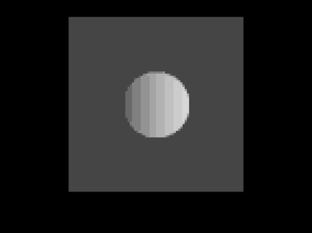

The Gaussian gets a different answer to the same picture, and not by a little. A kernel has no notion of inside, so what it reports at the centre depends on how far the rim is compared with σ; on a ring several σ across it reports almost nothing at all, and what it does report carries a gradient across the middle from the bright side to the dim one.
That gradient is the signature of the wrong model, and it is testable by anybody with a stabilised image and a patient observer: a filled region is uniform, and a blurred one is not.
What a disc actually does when it fades
The observation the phenomenon is named for is worth stating in the form the new model reproduces, because the old one reproduced only half of it.
A stabilised disc does not dim. Its interior takes the colour of the ground around it while its border stays put, and after a few seconds the disc is gone and the ground is continuous. Then a blink or a small movement brings it back instantly.
The old model gets the first half: everything coarser than the pool goes, and the disc’s interior is coarse while its border is not, so what remains is an outline. What it cannot say is what the interior becomes. Blurring a disc gives a disc with soft edges, which is not what anybody reports.
The new model says the interior becomes the average of its own border — and since the border, once the disc has faded, is being driven by whatever surrounds it, the average is the ground. The disc takes the colour of the ground because the ground is what its border is touching, and that sentence is a derivation rather than a description.
The instant recovery on a blink follows too, and is the one part that needs no new machinery. The signal is held on the border cells; move the image and the border cells change; the interior re-solves in the time a diffusion takes to cross the region, which for a small disc is short.
Two regions that share a contour
The interesting consequence of a boundary average rather than a neighbourhood average is what happens when two regions meet.
Under a kernel, two adjacent regions bleed into each other in proportion to how close they are, so a thin region takes on a great deal of its neighbour and a thick one takes little. Under a bounded diffusion they do not interact at all: each is bounded by its own contour, each settles to the mean of its own border, and their filled values are independent of one another and of their sizes.
That is a sharper claim than it sounds, because it says the area of a region has no effect on its steady-state filled value — only on the time it takes to get there. A speck and a wall bounded by identically driven borders fill to the same value.
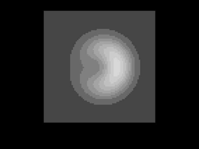
The experimental version is simultaneous contrast, which this collection has already measured as an appearance effect, and the two accounts are not the same thing: simultaneous contrast is about a patch that is present, and filling-in is about one that is not. What the model here says is that when a patch has faded, the mechanism that decides what stands in its place is a boundary condition rather than a proximity weighting.
Why the difference is a difference of kind
It is tempting to read the two models as the same idea at different resolutions — a kernel is a crude diffusion, a diffusion is a fancy kernel — and for an unbounded field that is true. A diffusion with a leak, on an empty field, is a convolution with an exponential kernel, and the two models differ only in the kernel’s shape.
The contour is what makes them different in kind. A convolution is a fixed kernel applied everywhere; the diffusion’s kernel is a Green’s function of the region, and a region with a wall in it has a Green’s function that goes around the wall. No amount of adjusting a fixed kernel produces that, because the operation the eye is being credited with is not the same operation.
The distinction has a name in the literature it comes from. Filling-in as a diffusion bounded by contours is the boundary-contour and feature-contour account of the 1980s, in which a boundary system computes where the edges are and a surface system spreads colour and brightness until it meets one. What is being added here is not the idea; it is the arithmetic, run on this collection’s own pool, with the predictions checked.

What it predicts that the old model does not
Three things, and the second and third are the neighbouring essay’s.
The interior is uniform. Not approximately — exactly, to the solver’s own tolerance, and independently of how the border varies. That is a strong prediction and it is the one a stabilised-image experiment can test most easily.
The interior’s value is a boundary average. So two regions sharing a contour need not agree, and a region’s filled colour is decided by its whole perimeter rather than by whatever is nearest.
And the clock belongs to the region. A diffusion fills a region in a time that grows with its area — proportionally, in the limit of a region large compared with the pool, and faster than that below it — so a large region fills slowly and a small one quickly, out of one set of constants. The old model has a single time constant and therefore predicts that a stabilised speck and a stabilised wall disappear together.
What the sixty per cent actually is
The kernel’s miss is quoted at 60 per cent of the border range. It is worth knowing what fixes that number, because it is not a property of either model.
Swept across ring radii, the bounded model’s centre error stays on the solver’s floor — between 8 × 10⁻¹¹ and 6 × 10⁻⁸ of the range, from a radius of 0.6° up to 2.5°, with no trend in it that is not the relaxation’s own tolerance. The kernel’s error moves: −0.555 at 0.6°, −0.577 at 1.0°, −0.600 at the 1.2° quoted, −0.625 at 2.0° and −0.625 at 2.5°.
It saturates, and the value it saturates at is arithmetic rather than perceptual. Once the ring is several pool widths across, a Gaussian sitting at the centre reaches essentially none of it, so the kernel reports nothing there and its error is the whole border mean. Written as a fraction of the border’s range, that is the mean divided by the range — and the test signal has a mean of 1 varying by 0.8 either way, so 1 divided by 1.6, which is 0.625 exactly.
The honest form of the comparison is therefore not a percentage but a statement about limits. For any region large compared with the pool, the kernel’s answer at the centre is zero and the bounded model’s is the border mean, whatever that mean happens to be. The 60 per cent is that difference expressed in the units of one ring at one radius, and a border that varied less would produce a larger number for the same disagreement.
That makes the gap easier to state and larger rather than smaller. The two models do not differ by a fraction of a signal. One of them reports a value and the other reports nothing at all, on every region wide enough to have an inside.
Making the signal vary less strongly around the ring is the check that the flatness inside is the boundary’s doing rather than the signal’s.
Whether the clock really goes as the area
The claim that a region fills in a time proportional to its area holds in a limit and not across the range these figures use, and the departure is worth having, because it is a check on the mechanism rather than a caveat about it.
Timing a disc’s centre to half its final value across radii from 0.4° to 2.8°, the local exponent relating time to radius falls monotonically: 3.23 at the smallest step, 2.86 at 0.7°, 2.58 at 1.0°, 2.40 at 1.2°, 2.24 at 2.0° and 2.17 at 2.8°. Proportional to area would be exactly 2, and the gate accepts anything between 1.9 and 3.0 for precisely this reason.
The trend is the right one and the reason is inside the model. A region whose radius is comparable to the diffusion length of 0.5° has a centre barely outside its own border’s near field, so what arrives there is governed by the source’s own falloff rather than by anything crossing the region — and that falloff is exponential, not diffusive. As the region grows past a few pool widths the crossing takes over and the exponent settles towards two.
So the prediction to put to an experiment is not “the time goes as the area” but “the time goes as the area for regions large compared with the pool, and steeper than the area for regions near its size”. Both halves are testable in one session, and the second is the more distinctive of the two: a stabilised speck does not merely fill faster than a stabilised wall, it fills faster than the ratio of their areas would allow.
What was computed, and how
The field is a square of stated extent in degrees of visual angle, discretised on an odd grid so that there is a centre cell. Two maps are laid on it: a permeability, which is one minus the contour strength, and a source, whose non-zero cells are held at their values.
The steady state is found by successive over-relaxation. The permeability between two neighbouring cells is the smaller of the two, so a single line of contour cells blocks rather than half-blocks — which is the difference between a wall and a curtain, and is the kind of detail that decides whether a model does what its description says.
The source ring sits just inside the barrier rather than on it, and that is the model rather than a convenience: a contour is impermeable, so a signal placed on one is a signal in a wall and reaches nowhere. The first version of this arithmetic did exactly that and filled every disc with nothing.
The mean value claim is asserted against the range of the border signal rather than against its mean, because a claim accurate to one per cent of a quantity that varies by eighty per cent is a claim about nothing. It comes out at 8 × 10⁻⁹ of the range, which is the relaxation’s own convergence tolerance rather than anything about the grid; the assertion is nevertheless set at two per cent, because the ring is two cells thick and its mean is a discretisation of an integral that a coarser field would not reproduce so exactly.
Cutting a gap in the contour is the case worth drawing next, because a real border is not a sealed ring and the slice is where a leak would show.

Where the two models agree, and why that matters
A new model that disagreed with the old one everywhere would be a different model rather than an extension, so it is worth being explicit about the overlap.
On an empty field they are the same operation up to the shape of a kernel. The assertion in the build takes a signal held along a line, with no contour anywhere, and measures how far it reaches: the value falls by a factor of e at a distance the equation makes equal to σ, and the measurement returns 0.484° against a stated 0.5°. A line source rather than a point one, because in two dimensions a point source is a Bessel function with a logarithm at the origin and reading a decay length off it measures the singularity.
On a stabilised grating they say the same thing. A grating has no enclosed regions, so there is nothing for a boundary to bound, and both models say the pattern survives to the extent it is finer than the pool. Every number in the fading essays about which spatial frequencies go and in what order is unchanged.
And the time constants are the same two. The clock is the two-pool state model this collection already had, not a third clock invented here. What the diffusion adds is a spatial time — how long the signal takes to cross a region — which multiplies the existing one rather than replacing it.
So the extension is conservative in the way a good one is: it changes the answers to questions the old model could not answer, and leaves the answers to the ones it could.
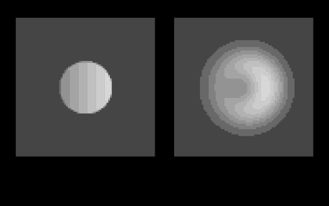
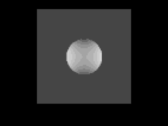
A signal with a second harmonic around the ring is the strongest test the construction admits, since it has two bright sides rather than one.
Where the model stops
The boundary map is an input. Where the contours are is given, not computed, so nothing here derives an illusory contour or explains why a stabilised edge survives when a stabilised gradient does not. What the model does is take a boundary as given and say what colour the region it encloses becomes, which is the half the phenomenon is named for.
No order between the channels. The equation is written once and run three times, so if colour goes before brightness it is not because of anything here. That absence is asserted, in the shape this collection uses for the effects its models deliberately do not predict.
And a stabilised image is not an ordinary one. The eye is never still, and drift is what stops the pool tracking in the first place. Everything here describes the limit in which the image is held fixed on the retina, which is an experimental preparation rather than a way of seeing.
The generalisation
A model that averages a neighbourhood and a model that solves a region give the same answer wherever there is no region, and different answers wherever there is one.
That is worth carrying because the first kind is very much easier to write and is what almost every implementation of a local operation actually is. A local contrast enhancement, a tone mapping operator, a denoiser, a white balance that varies across the frame — all of them are kernels, and all of them average across edges because a kernel does not know an edge is there. The visible artefact is the same in every case: a halo, which is exactly the gradient the wrong model leaves in the middle of a region.
The remedy is the same too, and it is why edge-aware filtering exists. What this essay adds is that the eye appears to be doing the region version, and that the difference is measurable in the one preparation where the eye can be made to hold still.
Where the ladder goes next
If a contour is a wall, a hole in it should let the surround in. It does not — the hole costs nothing at all while the border signal is unbroken, and what a gap actually costs is something else.
Where this goes next
 What a still eye stops seeing
A stabilised image is said to vanish, and nothing in a temporal filter predicts it — sensitivity at zero frequency is a quarter of the peak, not nothing. Give the adaptation gain a size and the answer falls out — fading is a high-pass filter that switches on over a minute, it takes the fill and leaves the outline, and a patch has to be about two degrees across before it goes at all.
What a still eye stops seeing
A stabilised image is said to vanish, and nothing in a temporal filter predicts it — sensitivity at zero frequency is a quarter of the peak, not nothing. Give the adaptation gain a size and the answer falls out — fading is a high-pass filter that switches on over a minute, it takes the fill and leaves the outline, and a patch has to be about two degrees across before it goes at all.
 A fading pool has a shape
Giving the local adaptation pool two axes instead of one costs a single parameter and produces a prediction the circular version cannot make — a stabilised grating fades at a rate that depends on which way its bars run. The obvious objection is the oblique effect, and the two act in bands that do not overlap.
A fading pool has a shape
Giving the local adaptation pool two axes instead of one costs a single parameter and produces a prediction the circular version cannot make — a stabilised grating fades at a rate that depends on which way its bars run. The obvious objection is the oblique effect, and the two act in bands that do not overlap.
 Brightness is inferred from edges
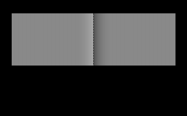
The Cornsweet effect makes two identical regions look different by altering nothing except a narrow band at the boundary between them. Cover the boundary and the difference vanishes, which says the visual system is reconstructing surfaces rather than reading off intensities.
Brightness is inferred from edges
The Cornsweet effect makes two identical regions look different by altering nothing except a narrow band at the boundary between them. Cover the boundary and the difference vanishes, which says the visual system is reconstructing surfaces rather than reading off intensities.
What this makes readable
Essays that name this one as a prerequisite.
Named alongside this one
Essays reaching for the same objects. Nobody chose these; they are what the index of named objects makes visible.
- What a second model changed assertion · colour appearance · spatial frequency
- A dark background moves every difference and no match colour appearance · simultaneous contrast
- A name in the model's own words assertion · colour appearance
- A patch is not a scene colour appearance · simultaneous contrast
- A viewing condition is a moment assertion · colour appearance
- An afterimage is an adaptation assertion · colour appearance
What links here
Every essay whose body links to this one.
The objects this essay names
Each one links to every other essay that touches it.
AssertionColour appearanceContourDiffusionFilling inLocal adaptationReceptive fieldSimultaneous contrastSpatial frequencyTroxler fading