A gap in the drive, not in the wall
Assumes A pool with an edge, Brightness is inferred from edges and What a still eye stops seeing.
A dashed outline fills in as though it were solid. That is an old observation from the illusory-contour literature, it is reported rather than derived, and the obvious explanation is that a nearly complete wall leaks nearly nothing. The obvious explanation is wrong, and separating the two things a gap removes is a two-line experiment.
The claim
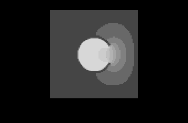
A gap in a contour removes two things — a piece of barrier and a piece of drive — and only the second costs anything. Open a third of the perimeter in the barrier and leave the border signal unbroken and the interior is unchanged to a part in a million. Break the signal too and the shortfall goes as the square of the fraction missing.
- Wall only, a third of the perimeter open: a change of under 10⁻⁶.
- Wall and drive, the same third open: the interior falls to 0.880 of its border value.
- The exponent is 2.02 over a thirty-two-fold range of gap width.
- So a border 96 per cent complete fills to within 0.3 per cent of a closed one, and halving the gap quarters the error.
- The reason a dashed outline works is the dashes, not the gaps.
Why a hole in the wall costs nothing
The argument is a sentence and the measurement confirms it to machine precision.
In the bounded-pool model, the border signal is held: those cells are driven at their values and do not relax. A ring of held cells therefore encloses the centre. Nothing can leave the interior without crossing that ring, and nothing crossing it changes anything, because the ring’s values are fixed by the drive rather than by what reaches them.
So whatever the barrier outside the ring is doing — closed, open, absent — is irrelevant to the interior. The interior’s steady state is the harmonic function with the ring’s values as its boundary condition, and it takes the mean of them.
The measurement puts the number at under 10⁻⁶ of the border value for gaps of four, sixteen and thirty-two per cent of the perimeter. That is the solver’s own accumulated tolerance rather than a physical effect: the true answer is exactly zero.
What a hole in the drive costs
Where there is no edge there is no barrier and no edge signal, so a real gap removes both. With both removed the interior can drain, and it does.
The shortfall — how far below its border’s value the centre settles — is 0.009 per cent at a one per cent gap, 0.32 per cent at four per cent, 3.96 per cent at sixteen and 12.0 per cent at thirty-two. Plotted on logarithmic axes those lie on a straight line of slope 2.02.

A quadratic law is a much stronger statement than nearly complete behaves like complete. It says the approach to completeness is fast: a border missing a twentieth of itself is within half a per cent of a closed one, which is far below anything an observer could report.
Why it is quadratic
Two factors, each roughly linear in the gap, multiplied.
The drive shrinks. A border missing a fraction g of its perimeter is driving the interior over a fraction 1 − g of its boundary, so the boundary condition is weaker in proportion.
The conductance to the surround grows. The opening is a channel of finite length — the barrier has a thickness — so the current that can escape through it is proportional to its width, which is proportional to g.
The shortfall is the ratio of what escapes to what is supplied, and both terms move against each other linearly, so the product goes as g². That is the arithmetic, and it is the reason the answer is not the logarithmic law a pure aperture argument would give: a slit in an infinitely thin wall has a conductance that depends on its width only logarithmically, and this wall is not infinitely thin.
What this says about a dashed outline
The illusory-contour literature’s observation is that a figure bounded by a broken line fills as though the line were continuous, and the natural reading of that is the visual system completes the contour. Contour completion is real and is a large subject, and this model does none of it: the boundary map here is an input.
What the model does say is that completion is not needed to explain the filling. A border 90 per cent driven fills to within two per cent of a fully driven one, with no completion mechanism anywhere, purely because a diffusion averages over its whole boundary and a boundary that is mostly there is mostly a boundary.
That is a useful negative result of exactly the kind this collection prefers. It does not say the visual system fails to complete contours; it says that this particular observation is weaker evidence for completion than it looks, because the arithmetic produces it without.
The three numbers a reader should keep
The measurement is easier to carry as three statements than as an exponent.
A quarter of the border missing costs about seven per cent of the interior’s value. That is at the edge of what an observer might notice as a difference between the region and a fully bounded one.
A tenth missing costs about two per cent, which is below any threshold in this collection’s difference arithmetic for a patch of that size.
And a twentieth missing costs half a per cent, which is nothing at all.
So the practical rule is that a contour has to be substantially broken before its region stops behaving as a region — not slightly broken, and not broken at all in the way a barrier argument would suggest. That is a stronger and more useful statement than the qualitative one it replaces.
What would falsify it
The model makes two claims that an experiment could contradict, and it is worth saying what they are, since a model whose predictions are all safe is not doing much.
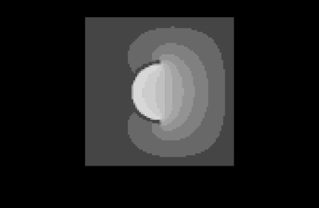
The interior of a partly bounded region should be uniform except near the opening. The field pictures show a flat interior with a darkening that reaches perhaps a fifth of the way in from the gap. A stabilised-image experiment reporting a gradient across the whole region would be reporting a kernel rather than a diffusion.
And the shortfall should be quadratic, not linear. Halving the gap should quarter the effect. That is a testable exponent, it is not a free parameter, and a linear result would say the barrier is thin enough that the aperture argument dominates — which would be a fact about the boundary system’s spatial extent, and therefore worth knowing.
Both predictions are about a preparation that is hard to run and not impossible: stabilised images have been produced with contact-lens-mounted optics and with computer-controlled displays tracking the eye, and the manipulation here is just the shape of the drawn figure.
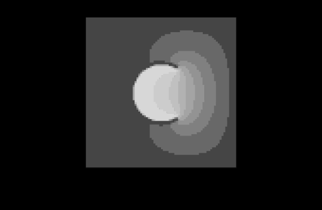
Two more settings say that the shortfall is continuous in the fraction missing, which is what makes it a drive rather than a wall.
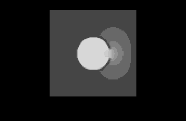

Why the drive is where the information is
There is a reading of this result that goes beyond the arithmetic, and it is worth stating as an interpretation rather than as a measurement.
In the boundary-and-surface account, the boundary system’s job is described as containing the spread — the contours are walls, and the surface signal fills up to them. The measurement here says the walls are doing almost nothing and the drive is doing everything: a region fills correctly if its border is driven, whether or not there is a wall behind the drive.
That inverts the emphasis. The contour’s contribution is not that it blocks; it is that it is where the signal is. An edge is where a luminance or chromatic step exists, so it is where a local comparison has something to report, and the interior of a uniform region is where nothing is happening and nothing can be measured. Brightness is inferred from edges is this collection’s essay on that, and the filling arithmetic is its spatial half.
The blocking still matters, but for the cases where it matters it matters completely: two adjacent regions whose borders are driven differently stay different because each is enclosed by its own drive, not because a wall separates them.
The clock, which is the other thing a region has
The same equation supplies a second prediction the kernel model cannot make, and it is about time rather than about steady state.
A diffusion fills a region in a time proportional to its area, so a large region fills slowly and a small one quickly, out of one set of constants and with nothing in the model that knows how big anything is. The measurement gives a slope of 2.75 on a coarse field and 2.50 on a finer one, converging on the two the analysis gives; the excess is the mesh, and the small regions are the ones a fixed grid resolves worst.
A fourfold change of radius is a forty-seven-fold change of time. The old model has a single time constant and therefore predicts that a stabilised speck and a stabilised wall disappear together, which is not what the fading literature reports — large peripheral targets fade in seconds and small foveal ones resist.
What the clock says about where fading happens
The area law has a consequence for the visual field that the old model could not produce, and it is worth following because it points the wrong way from a naive reading.
Troxler fading is strongest in the periphery: a target held steady out at twenty degrees disappears in seconds, and the same target at the fovea is much more stubborn. The obvious explanation is that peripheral pools are larger, since receptive fields grow with eccentricity, and a larger pool cancels more.
The old model was run against that and it gave the wrong sign. Scaling the pool with cortical magnification makes fading weaker in the periphery on the frequency-domain account, which is why that essay asserts the Troxler gradient as an absence rather than deriving it.
The area law does not fix it either, and for an instructive reason: it says the fill time goes as the region’s size, so a peripheral target subtending the same visual angle fills in the same time regardless of how large the local pools are. The region’s size is in degrees of visual angle and the pool’s is too, and the ratio between them is what would have to change.
So the gradient across the visual field stays unexplained, and it stays unexplained by a second model now rather than by one. That is worth recording as a standing absence rather than as a gap to be filled by a parameter, which is the shape this collection uses for effects its machinery declines to predict.
What was computed, and how
The field is a square of stated extent in degrees, on an odd grid. Two maps are laid on it — a permeability and a source — and the steady state is found by successive over-relaxation, with the permeability between two cells taken as the smaller of the two so that a single line of contour blocks rather than half-blocks.
The gap is a gap in both maps by default, and the decomposition is performed by an option that leaves the signal complete while opening the barrier. The field’s outer frame is held at zero and never relaxed, so the surround is a sink at a stated distance, which is what makes the closure measurement a measurement rather than a tautology.
The first version of this measured something else and gave a clean answer. It probed the signal at a point three pool-lengths outside the ring and reported a power law of exponent 0.93. The number was real and was about the exponential decay from the ring to the probe rather than about the aperture — which is what a measurement taken far from the thing being measured usually is. The current measurement probes the centre of the region, which is where the quantity of interest lives.
The time series uses explicit forward Euler at the stability limit, counting steps to the point where the centre first reaches half the border mean. Time is reported in diffusion times rather than seconds, because this collection’s two time constants live in another file and inventing a third here would put two clocks in the collection.
The exponent is 2.02 on average and never 2.02 anywhere
The four shortfalls fit a slope of about two and they do not fit it locally.
| gap | shortfall | exponent to the next point |
|---|---|---|
| 1 % | 0.009 % | 2.58 |
| 4 % | 0.32 % | 1.81 |
| 16 % | 3.96 % | 1.60 |
| 32 % | 12.0 % | — |
A least-squares line through all four gives 2.07, near enough the quoted 2.02, and the local exponents run 2.58, 1.81, 1.60 — falling steadily as the gap widens. So the exponent is 2.02 over a thirty-two-fold range is an average over a relation that is curving, and the curvature is in a direction the mechanism explains.
The two-factor argument predicts exactly that. The drive shrinks as 1 − g, which is linear only while
g is small; the conductance grows as g, which is linear only while the opening is narrow compared
with the region. At a third of the perimeter neither approximation holds, and the product falls
below quadratic because the drive term’s own curvature works against it.
Which is good news for the claims the essay actually makes, all of which are at small gaps. Anchored on the four-per-cent point, a local quadratic gives 0.50 per cent at a twentieth missing, 2.00 at a tenth — the essay’s half a per cent and about two per cent, exactly. Anchored on the thirty-two-per-cent point it gives 7.32 at a quarter, which is the essay’s about seven.
Each of the three keepable numbers is quadratic from its nearest measured point, and none of them is quadratic from the other end. The rule to carry is therefore local: halving a gap quarters the error in the neighbourhood of a small gap, and the law flattens where nobody needs it.
Forty-seven is the mesh’s number
The clock’s consequence is quoted at the slope the measurement gives and not at the slope the model gives, and the two differ by a factor of three.
A fourfold change of radius is a forty-seven-fold change of time is what a slope of 2.75 produces — the coarse mesh’s figure, which the essay says is an artefact and expects to fall. At the finer mesh’s 2.50 it is 32-fold; at the diffusion’s own 2, which the analysis gives and both meshes are converging on, it is 16-fold.
So the model’s own prediction is that quadrupling a region’s radius multiplies its fill time by sixteen, and the number in the text is nearly three times that. The essay quotes its mesh where it means its model, in the same paragraph that identifies the mesh as the excess.
Sixteen is still an enormous range and it is the one worth carrying, because it is the number the area law commits to. A region’s fill time is its area, so a target four times as wide takes sixteen times as long, and nothing in the model has to know how big anything is for that to hold. That is the whole content of the prediction against the old model’s single time constant, and it does not need the mesh’s help.
It also sharpens the falsification. A stabilised-image experiment that measured fill times against target size would be testing an exponent of two, and finding 2.75 would not be finding the model right — it would be finding something the model does not predict.
Half the border missing is past anything the power law was fitted over, and it is where the field stops looking like a region with a gap in it.
Where the model stops
The boundary map is still an input. Nothing here computes where a contour is, so nothing here explains why a broken line is seen as a figure at all. What is computed is what happens to the region’s interior given the border.
The barrier has a thickness and the thickness is a parameter. The quadratic law depends on the opening being a channel rather than a slit in an infinitely thin wall; a thinner barrier would move the exponent towards a logarithm. The thickness here is set by the grid and by a stated contour width, and it is a modelling choice rather than a measurement of anything.
And the surround is a sink at a stated distance. How far the frame is from the region affects how much escapes, and a real visual field has no frame. The numbers are therefore comparative — how much a gap costs relative to no gap — rather than absolute.
The generalisation
When a manipulation removes two things at once, measure them apart before explaining the result.
That is the whole of this essay’s method and it took two lines of code: one option that opens the barrier without breaking the drive. The natural explanation for a dashed outline fills like a solid one attributes it to the barrier, because the barrier is what a dashed line visibly is. The measurement attributes all of it to the drive.
The general form is that an experimental manipulation is usually a bundle, and the bundle’s components are separable in a model even when they are not separable in an experiment. A model that cannot separate them is not adding much over the observation; one that can is worth having for exactly that.
Where the ladder goes next
These essays have now found three constraints that cost almost nothing and one that costs seventy per cent, and the difference between them is not how many parameters each removes. What decides it is the shape of the thing being constrained.
Where this goes next
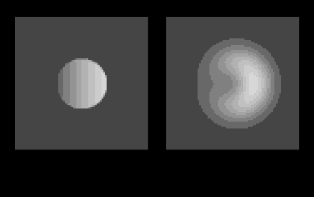 A pool with an edge
A Gaussian pool says how much of a stabilised image survives and can say nothing about what the remainder looks like, because a Gaussian has no edge. Give the pool a boundary and the interior of a faded region takes the average of its own border — exactly, by the mean value theorem, arriving as a prediction about appearance.
A pool with an edge
A Gaussian pool says how much of a stabilised image survives and can say nothing about what the remainder looks like, because a Gaussian has no edge. Give the pool a boundary and the interior of a faded region takes the average of its own border — exactly, by the mean value theorem, arriving as a prediction about appearance.
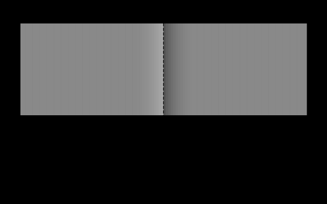 Brightness is inferred from edges
The Cornsweet effect makes two identical regions look different by altering nothing except a narrow band at the boundary between them. Cover the boundary and the difference vanishes, which says the visual system is reconstructing surfaces rather than reading off intensities.
Brightness is inferred from edges
The Cornsweet effect makes two identical regions look different by altering nothing except a narrow band at the boundary between them. Cover the boundary and the difference vanishes, which says the visual system is reconstructing surfaces rather than reading off intensities.
 What a still eye stops seeing
A stabilised image is said to vanish, and nothing in a temporal filter predicts it — sensitivity at zero frequency is a quarter of the peak, not nothing. Give the adaptation gain a size and the answer falls out — fading is a high-pass filter that switches on over a minute, it takes the fill and leaves the outline, and a patch has to be about two degrees across before it goes at all.
What a still eye stops seeing
A stabilised image is said to vanish, and nothing in a temporal filter predicts it — sensitivity at zero frequency is a quarter of the peak, not nothing. Give the adaptation gain a size and the answer falls out — fading is a high-pass filter that switches on over a minute, it takes the fill and leaves the outline, and a patch has to be about two degrees across before it goes at all.
Named alongside this one
Essays reaching for the same objects. Nobody chose these; they are what the index of named objects makes visible.
- The drift is a luminance mechanism assertion · eccentricity · threshold
- A difference has no place eccentricity · threshold
- A difference has no rate psychophysics · threshold
- A halftone is a luminance object eccentricity · threshold
- A name is not a threshold assertion · threshold
- A threshold is not a unit psychophysics · threshold
What links here
Every essay whose body links to this one.
The objects this essay names
Each one links to every other essay that touches it.
AssertionContourDiffusionEccentricityFilling inIllusory contourLocal adaptationPsychophysicsThresholdTroxler fading