Three cones, two axes
Assumes Three numbers and Why colour is exactly three-dimensional.
Three receptors produce three numbers. The obvious thing to do with three numbers is send them somewhere, and the retina does not do the obvious thing.
What leaves the eye is a sum and two differences, and the transformation between them is the most consequential piece of arithmetic in the visual system — everything from the four unique hues to the shape of colour blindness to the axes of CIELAB descends from it.
The redundancy the recoding removes
The L and M cones peak near 564 and 534 nanometres. That is thirty nanometres apart on curves more than a hundred nanometres wide, so the two overlap almost completely.
Run a family of natural reflectances under daylight through both, and their responses correlate at 0.999. Knowing one is very nearly knowing the other.
Sending three such signals down the optic nerve would spend two channels carrying one quantity. The optic nerve is a genuine bottleneck — about a million fibres for a hundred and twenty million receptors, most of them rods — so the pressure to not waste it is real, and this is the classic case of it.
Deriving the axes rather than quoting them
The standard presentation gives the opponent channels as definitions: luminance is L+M, red-green is L−M, blue-yellow is S−(L+M). They are usually presented as facts about physiology, established by recording from cells.
They can be derived instead, and the derivation is more informative than the citation.
Take a family of smooth reflectances spanning what the world contains. Run them through the cone fundamentals. Take logarithms, because receptor response is compressive and the redundancy being removed is multiplicative. Compute the covariance and find its eigenvectors — the three directions along which the data varies independently.
What comes out is not chosen and not fitted:
- An axis weighting the three cones at 0.576, 0.579, 0.577 — equal to two decimal places. An achromatic channel.
- An axis at −0.475, −0.336, 0.813. S against the sum of L and M. Blue-yellow.
- An axis at −0.665, 0.743, −0.081. L against M, with almost no S. Red-green.
Nothing in the calculation knows what a colour channel is. The opponent structure falls out of the statistics of natural spectra, and the eye’s job was to notice.
This is Buchsbaum and Gottschalk’s result from 1983, and it is one of the most satisfying in the subject: a physiological arrangement explained by the properties of the environment it evolved in, with the explanation checkable in a few lines of arithmetic.
The ordering, which is not the expected one
The three channels carry 97.1%, 2.85% and 0.012% of the variance.
The last of those is red-green, and it is the surprising one — because red-green is the channel everybody means by “colour”. It is the one colour blindness is usually about, the one CIELAB writes first, the one the word mostly refers to in ordinary speech. Across natural spectra it carries one part in ten thousand, three orders of magnitude below blue-yellow.
The first version of the check in this site’s gate demanded red-green second, on the strength of that intuition. It failed, and the measurement was right. The check now requires the ordering achromatic, blue-yellow, red-green, and requires red-green to be at least twenty times smaller than blue-yellow — asserted in that direction, because the ordering is the finding.
The reason is the correlation above. L and M are nearly the same measurement, so their difference is nearly nothing. A channel built from a difference between two near-identical signals has almost no signal in it.
What makes it worth building anyway is that “almost nothing” is not nothing, and the little that is there is useful. The L and M difference is what separates ripe fruit from leaves, and the standard account of why old-world primates re-evolved trichromacy is exactly that. A channel carrying one part in ten thousand of the variance was worth a gene duplication because of which part.
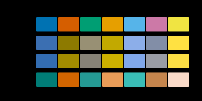
What a channel carrying one part in ten thousand is actually worth can be seen by removing it, which is what protanopia does and what the construction below simulates on a palette chosen to be distinguishable.
What the second stage explains
Several facts that make no sense at the receptor level become straightforward once the recoding is in place.
There is no reddish green. A single channel cannot be positive and negative simultaneously, so a colour cannot be at both ends of the red-green channel. It can be at one end of each channel, which is why reddish blue and yellowish green are ordinary. This is the strongest structural prediction opponent theory makes, and it is a prediction about a class of experiences rather than a number.
There are four unique hues. Two chromatic channels with two ends each. Where exactly they land is a harder question the theory answers less well.
Afterimages are complementary. Fix on red, look away, see green. Adaptation in an opponent channel drives it toward its opposite end, which a receptor-level account has to work considerably harder to produce.
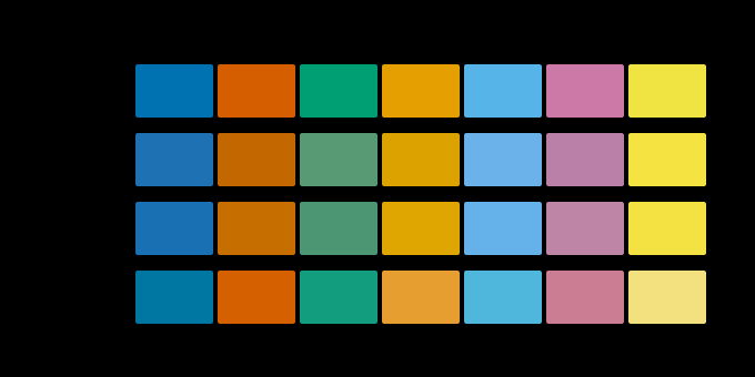
Colour deficiency comes in the shapes it does. Losing L or M collapses the channel built from their difference, which is why the common deficiencies are red-green. Losing S — far rarer, and not sex-linked — collapses the other. The simulation is a projection onto the surviving channels.
Chromatic and achromatic resolution differ enormously. The achromatic channel carries nearly all the variance and is sampled finely; the chromatic channels are pooled far more heavily. This is why image and video compression can discard most of the chroma resolution and why nobody notices — chroma subsampling is an engineering exploitation of the second stage, arrived at empirically decades before the justification was available.
What compression already knew
The clearest practical evidence for the variance ordering is a piece of engineering that predates the measurement by decades.
Every image and video format in use discards most of the chromatic resolution and keeps the luminance resolution. JPEG converts to a luma-plus-two-chroma representation and subsamples the chroma; every video codec does the same, usually more aggressively, throwing away three quarters of the chroma samples. Nobody notices.
That works because the achromatic channel carries nearly all the variance and is sampled finely by the visual system, while the chromatic channels are pooled far more heavily in the retina and carry far less. A codec discarding chroma resolution is exploiting the second stage, and the arrangement was arrived at empirically — by people finding what could be thrown away without complaints — long before the information-theoretic justification existed.
The colour space every codec uses for this is a luma-chroma transform of RGB, and it is worth noticing that it is not the opponent basis derived above. It is a fixed matrix chosen for computational convenience and standardised in the 1950s for analogue television compatibility. It is opponent-shaped — one weighted sum and two differences — and it is not the decorrelating transform.
That it works nearly as well is the useful lesson. The decorrelation result says the achromatic direction dominates and the chromatic directions are small; any transform that separates a weighted sum from two differences captures most of the benefit, and the exact weights matter far less than the structure. Which is also why CIELAB’s opponent-shaped axes are useful while not being the opponent channels.
Hering and Helmholtz were both right
The nineteenth-century dispute is usually taught as a contest with a winner, and it was not.
Helmholtz, following Young, argued for three receptor types. Hering argued that colour experience is organised around opposed pairs — red against green, yellow against blue, black against white — and pointed at exactly the phenomena above: no reddish green, four elementary hues, complementary afterimages.
The arguments were treated as incompatible for eighty years. They describe consecutive stages. Three receptors feed two chromatic channels and one achromatic one, Helmholtz was right about the first stage, Hering about the second, and the resolution arrived in the 1950s when Hurvich and Jameson measured opponent responses directly.
The lesson generalises past colour. Two well-supported theories that appear to contradict each other are sometimes describing different levels of the same system, and the question “which is right” was the wrong question for eight decades.
Where CIELAB fits, and does not
CIELAB’s a* and b* axes are constantly described as the red-green and yellow-blue axes, and the description is an inheritance from this stage.
It is not accurate. If a* were the red-green axis, the four unique hues would sit at 0°, 90°, 180° and 270°; they sit at 25°, 88°, 161° and 250°. The axes were constructed to be roughly opponent-shaped and are not the opponent channels, and treating them as such — a quadrant test for hue category, a “warm or cool” heuristic — places boundaries twenty-odd degrees from where observers put them.
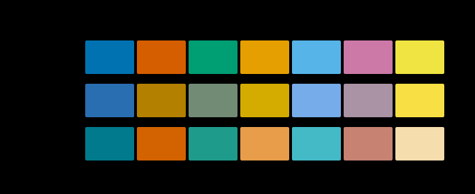
The two chromatic channels can also be removed one at a time and at partial strength, which separates the question of which channel is lost from the question of how completely.
The one receptor that has nothing to decorrelate
A useful contrast: none of this applies to rod vision, and the reason is instructive about what the second stage is for.
Rods have one pigment. One receptor type produces one signal, one signal has no redundancy with anything, and there is nothing for an opponent stage to remove. Rod vision therefore has no chromatic channels, which is the same statement as saying it has no colour — not a deficiency of the rod pathway but a straightforward consequence of there being one of it.
This puts the trichromatic case in perspective. Three receptors are not three sources of information about colour — they are three heavily overlapping measurements of the same spectrum, from which a small amount of chromatic information can be extracted by differencing. The extraction is the second stage’s whole job, and the amount extracted is, by the measurement above, about 3% of what arrives.
The rest is luminance, and luminance is what a single receptor type already gives. Colour is the residual.
The loss is graded rather than binary, since an anomalous trichromat has a shifted pigment rather than a missing one, so the same construction at a third of full severity is closer to what most affected people carry.
What was computed here
The reflectances are constructed rather than measured, and the essay says so. They are a family of smooth curves with three degrees of freedom — level, slope and curvature — walked over a lattice.
That is an honest caricature of a real property: measured collections of natural reflectances turn out to need about three basis functions to reconstruct to within measurement error, which is a remarkable fact and not one the eye had any say in. A measured collection would be better and this site does not have one.
The eigendecomposition is by cyclic Jacobi rotation, written out rather than approximated, because the whole argument is that specific axes fall out of the data — an iterative method that stopped early would produce axes that were nearly right and prove nothing. Each eigenvector’s sign is fixed so its largest entry is positive, since an eigenvector is only defined up to a flip and nothing downstream would be comparable otherwise.
Each axis is classified from its own weights rather than from where it landed in the ordering. An eigenvector with three same-signed entries is achromatic wherever it came out; one setting L against M with little S is red-green. The classification is a test the vectors can fail, not a label applied to whichever axis came second.
Three things are asserted. L and M must correlate above 0.99, because without that redundancy there is nothing for the recoding to remove. The three axes must classify as achromatic, blue-yellow and red-green in that order. And the achromatic axis must weight the three cones within 0.05 of each other, since an achromatic channel that weighted them unequally would not be one.
The printed vectors are an orthonormal basis
The three eigenvectors are quoted to three decimals and it is worth checking that the printed numbers still are what they claim to be, because a reader has no other access to the computation.
Each has unit length to within 0.0004, and each pair is orthogonal to within 0.001. So the nine printed numbers really are three perpendicular directions of unit length — the object an eigenanalysis of a symmetric matrix returns — and nothing has been rounded past the point of being one.
That matters more here than in most tables, because the essay’s claim is that the axes fall out rather than being chosen. A set of weights that failed orthogonality would be a set somebody had adjusted.
Two point four orders, not three
Three orders of magnitude below blue-yellow is the essay’s summary of the red-green channel, and the three variances give a different gap.
97.1, 2.85 and 0.012 per cent put red-green 238 times below blue-yellow — 2.4 orders — and 8,092 times below achromatic, which is 3.9. So the three-orders figure sits between the two comparisons and belongs to neither.
The correction runs the same way as the finding. Red-green is nearly four orders below the achromatic channel, which is a larger gap than the essay claims for it against blue-yellow, and the surprising comparison is the one the essay does not make: the channel everybody means by colour carries one eight-thousandth of what the channel nobody thinks of as colour carries.
And the pair together carries 2.862 per cent, which is the about 3 per cent quoted later — so the two chromatic channels are 3 per cent and the red-green one is 0.4 per cent of that 3 per cent. Colour is the residual, and red-green is a residual of the residual.
The correlation is quoted a decimal short
The red-green channel is small because L and M correlate, and the two numbers do not quite fit.
For a pair correlating at r, the smaller of the pair’s own two principal components carries
(1 − r)/2 of their joint variance. At the quoted 0.999 that is 0.05 per cent — four times the
red-green channel’s measured 0.012 per cent of the whole.
Since the L and M cones carry very nearly the whole variance between them, the two should agree, and they do at a correlation of 0.9998 rather than 0.999. Quoting the correlation to three decimals understates the redundancy by a factor of four, and the fourth decimal is where the argument lives: 0.999 and 0.9998 are the same number to a reader and a factor of four to the channel built from their difference.
That is worth stating because the correlation is the essay’s mechanism and the variance is its finding, and a reader checking one against the other with the printed figures will not reproduce it. A quantity whose consequence is a difference needs one more digit than a quantity whose consequence is a sum, and this is the cleanest instance of that rule in the collection.
Sixteen degrees, not twenty-odd
The CIELAB section quotes the four unique hues at 25°, 88°, 161° and 250° against axes at 0, 90, 180 and 270, and calls the discrepancy twenty-odd degrees.
The four deviations are +25, −2, −19 and −20, so the mean absolute displacement is 16.5 degrees and one of the four — yellow, at 88 against 90 — is essentially on its axis.
So the failure is not uniform and it is worth knowing which axis works. Yellow sits where b*'s positive end is; blue sits twenty degrees off b*'s negative end; and the two ends of a* are off by 25 and 19 in opposite senses, so a* is not merely rotated — its two ends disagree about which way.
That is a more specific complaint than the axes are not the opponent channels. One half-axis of the four is right, and the a* axis is not a straight line through the unique hues at all — a rotation could fix a common offset and cannot fix two ends that need moving in opposite directions.
Where the model stops
This is an argument about why the recoding exists, and it is not a model of the retinal circuitry that implements it.
The real circuitry is not a clean matrix multiplication. Horizontal and amacrine cells build centre-surround receptive fields that mix spatial and chromatic opponency together, so the “red-green” cells in the primate retina are simultaneously edge detectors — a single cell’s response confounds a chromatic difference with a spatial one, and separating them is an unsolved problem in visual neuroscience.
The decorrelation argument also predicts the axes and not their weights in perception. The eigenvectors say which combinations are independent; they do not say how the visual system scales them afterwards, and it does scale them, substantially.
And the derivation depends on the input statistics. Different reflectance families give slightly different axes. What is robust is the structure — one achromatic channel dominating, an S-opposed channel second, an L−M channel far behind — and not the third decimal place of any weight.
What the pictures cannot show
The scatter plots show cone responses, which nobody experiences. There is no figure here of what an opponent channel looks like, because an opponent channel does not look like anything: it is a signal on a nerve, and what it contributes to is an experience that also involves the other two.
The bar chart is on a log scale, and that is a real distortion in service of legibility. On a linear scale the achromatic bar would fill the figure and the other two would be invisible — which is a truer picture of the proportions and a useless one. Any reader taking a visual impression of relative magnitude from that figure is reading a logarithm, and the numbers are printed for exactly that reason.
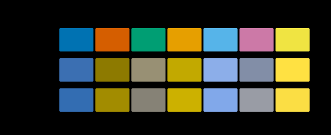

The severity of the loss is a dial rather than a switch, and most people who have one of these are somewhere along it.
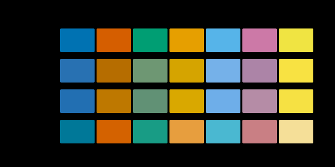

All three collapses together on the palette this site checks its own figures against are what say the two axes are two rather than one or three.
Who found it, and when
Hering published his opponent account in the 1870s, from phenomenology — the impossible colours, the elementary hues, the afterimages — and was largely dismissed by the physiologically-minded majority.
Hurvich and Jameson vindicated him in the 1950s with hue cancellation: to measure how much redness a stimulus contains, let an observer add green until the redness is exactly cancelled, and the amount added is the measure. It converts an introspective report into a null measurement, which is the same trick colour matching uses and is why both are quantitative.
Svaetichin recorded from horizontal cells in fish retina in 1956 and found cells responding with opposite sign to different wavelengths — the first direct physiological evidence, and found in a fish because primate retina is considerably harder to record from.
Buchsbaum and Gottschalk gave the information-theoretic derivation in 1983. Ruderman, Cronin and Chiao extended it to natural images in 1998 and established the variance ordering — including the finding that the L−M axis carries least, which remains the least-quoted robust result in the field.
Where this goes next
The four hues the two chromatic channels produce, and the awkward question of where exactly they sit, is why there are four unique hues. The receptors feeding all of this are three numbers. And the dimension count that this stage preserves while redistributing what each dimension carries is why colour is exactly three-dimensional.
Where this goes next
 Three numbers
A spectrum has as many degrees of freedom as anyone cares to give it. The eye reports three. Everything colour science can do, and every way it fails, follows from that one collapse.
Three numbers
A spectrum has as many degrees of freedom as anyone cares to give it. The eye reports three. Everything colour science can do, and every way it fails, follows from that one collapse.
 Why there are four unique hues
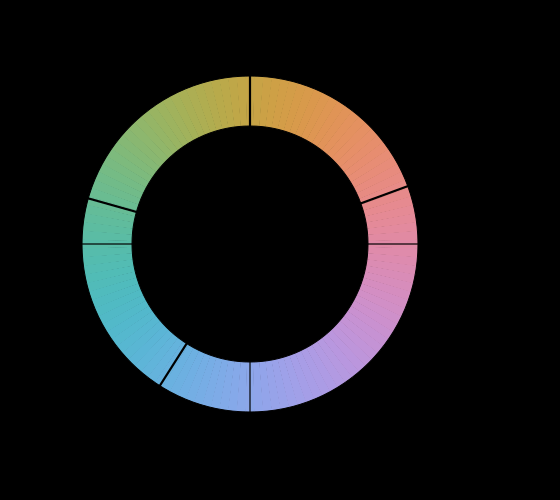
Observers agree that four hues are elementary and that no colour is reddish green. Nothing in the three receptors predicts either fact, and the axes of every standard colour space miss the four by tens of degrees.
Why there are four unique hues
Observers agree that four hues are elementary and that no colour is reddish green. Nothing in the three receptors predicts either fact, and the axes of every standard colour space miss the four by tens of degrees.
 Why colour is exactly three-dimensional
Matching every wavelength with three primaries requires, for some wavelengths, a negative amount of one of them. That physical awkwardness is why the colour-matching functions were transformed into XYZ, and why the horseshoe is curved.
Why colour is exactly three-dimensional
Matching every wavelength with three primaries requires, for some wavelengths, a negative amount of one of them. That physical awkwardness is why the colour-matching functions were transformed into XYZ, and why the horseshoe is curved.
What this makes readable
Essays that name this one as a prerequisite.
Named alongside this one
Essays reaching for the same objects. Nobody chose these; they are what the index of named objects makes visible.
- A difference has no place cielab · opponent processing
- The colour is in the thickness cielab · reflectance
- The drift is a luminance mechanism opponent processing · second stage
- White turns a hue, and the models part at blue cielab · unique hues
What links here
The 8 essays that link to this one and share the most of its objects, of 16 that link here.
The objects this essay names
Each one links to every other essay that touches it.
CIELABCone correlationDecorrelationEfficient codingHering's opponent theoryOpponent processingReflectanceSecond stageUnique hues