The hue scale has four corners
Assumes An appearance is not always a stimulus, Why there are four unique hues and The appearance model takes XYZ.
Every quantity CIECAM16 reports is a formula except one. Lightness, brightness, chroma, colourfulness and saturation are algebraic expressions in the compressed cone signals — six numbers the situation moves very unequally. Hue quadrature is a table with four rows in it and an interpolation between them.

The claim
The model’s hue scale is an interpolation through four measured numbers, so it has a corner at each of them and runs four times faster in one place than in another.
- Its slope jumps at every anchor: by a factor of 1.19 at red, 1.18 at yellow, 1.74 at green and 0.41 at blue.
- Across the circle the slope runs from 0.47 near hue 238 to 1.92 near hue 90, a factor of 4.1.
- The quadrant from blue back to red spans 142.6 degrees of hue angle for its hundred units of quadrature, against 69.9 for red to yellow.
- And a tolerance stated in quadrature is therefore four times tighter in one place than in another, in the units anybody would measure the match with.
What quadrature is for
The model reports hue as an angle in its own opponent plane, and that angle is a computed quantity with no perceptual claim attached: it is the arctangent of a ratio of two signals, and where its zero falls is an accident of the matrix.
Hue quadrature exists because observers do not agree with that. Four hues are elementary — a red that is neither yellowish nor bluish, and three others — and the fact that they are is one of the oldest results in the subject and is not predicted by anything in three receptors. An appearance model that reported only an angle would be reporting a number whose zero meant nothing to anybody, in the way CIELAB’s axes are not the unique hues.
So the model carries four measured anchor hues with four fitted weights and interpolates between them. Red is at hue angle 20.14 and quadrature 0; yellow at 90.0 and 100; green at 164.25 and 200; blue at 237.53 and 300. The interpolation is a ratio of two linear expressions — a hyperbola rather than a straight line — with each anchor’s weight in it.
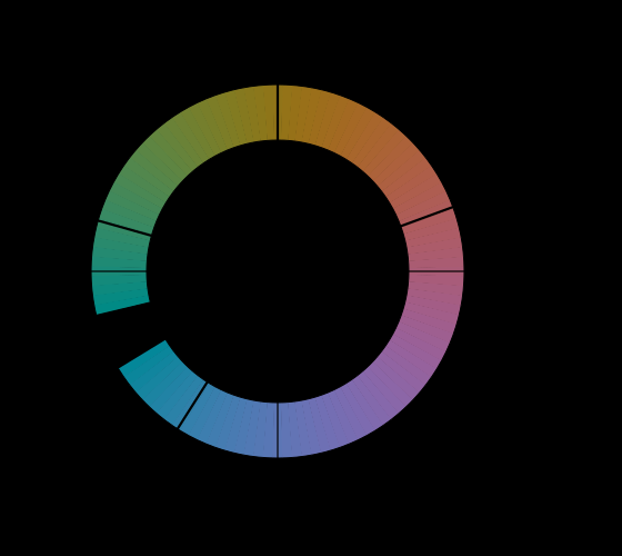
That is a reasonable design and it is the only one available: four measurements and a rule for the space between them. What it produces is a function with the properties an interpolation has, and those properties are not usually stated.
Why an interpolation rather than a fit
The obvious alternative is to fit a smooth function to the four measurements rather than to interpolate through them, and it is worth saying why the standard does not.
A fit through four points with a smooth function has one property the standard cannot accept: it does not pass through the points. Whatever it does at hue angle 90, it will not report exactly 100 units of quadrature there, and 100 at unique yellow is not an empirical claim to be approximated — it is the definition of the scale. Quadrature is constructed so that the four unique hues fall at 0, 100, 200 and 300, and a scale that put unique yellow at 99.4 would have given up the thing it exists for.
So the choice is between exactness at four points with corners, and smoothness everywhere with the anchors slightly wrong. The standard chose exactness, which is correct, and the corners are what that costs.
There is a third option nobody took, which is to keep the anchors exact and choose an interpolation with matching slopes — a cubic through four points with derivative conditions, say. It has no corners and it needs derivative values at the anchors, and nothing measures those: an observer can say which yellow is unique and cannot say how fast hue changes there. A smooth scale would have required inventing four numbers, which is a worse fault than a corner and is presumably why it was not done.
What the weights are doing
The four anchors carry four weights — 0.8 at red, 0.7 at yellow, 1.0 at green, 1.2 at blue — and those are the numbers that produce most of the unevenness.
The interpolation divides the distance from the lower anchor by that anchor’s weight and the distance to the upper one by the upper anchor’s weight, and forms a ratio. So a large weight makes an anchor repel: the scale moves slowly near blue because blue’s weight is the largest, and quickly near yellow because yellow’s is the smallest.
The ratio between the extreme weights is 1.2 over 0.7, which is 1.71 — and the observed slope ratio across the circle is 4.1. The rest comes from the anchor spacing, which is uneven for a reason that is not fitted at all: there is no unique purple, so the gap from blue back to red is two-fifths of the circle carrying one quarter of the scale.
That decomposition is worth having because the two causes have different status. The weights are fitted parameters, so a different data set moves them. The absence of a fifth anchor between blue and red is a fact about human colour vision that no data set will move — there are four unique hues and there is no reddish green — so the largest single contribution to the scale’s unevenness is a structural feature of the eye rather than a modelling choice.
Where the corners are
An interpolation through four points, with a different formula in each of four intervals, is continuous at the joins and is not smooth there. The value matches; the slope does not.

At red the slope goes from 1.05 below the anchor to 1.25 above it, a factor of 1.19. At yellow, 1.64 to 1.92, a factor of 1.18. At green, 0.94 to 1.64, a factor of 1.74. At blue, 1.14 to 0.47, a factor of 0.41.
The blue anchor is the largest discontinuity and it is a drop, at the hue where the published adaptation transforms disagree most. Crossing hue angle 237.53 the scale more than halves its rate, so two colours a degree apart on the yellow side of blue are further apart in quadrature than two colours a degree apart on the other side by a factor of two and a half.
Nothing is wrong with that. It follows from the weights, the weights were fitted to data, and the data say the four unique hues are not evenly spaced in the model’s own opponent plane. The interpolation is doing what an interpolation does, which is to be exactly right at the nodes and to have a corner at each of them.
How unevenly it runs
The corners are local and the unevenness is global, and the global figure is the one a specification would care about.
Across the whole circle the slope runs from 0.468 units of quadrature per degree, just above blue, to 1.918 just above yellow. That is a factor of 4.1, and it means the quadrature scale is compressed by four times more in one part of the circle than in another.
The quadrant spans say the same thing more legibly. Red to yellow is 69.9 degrees of hue angle for 100 units of quadrature; yellow to green is 74.3; green to blue is 73.3. Blue back to red is 142.6 — twice the others, for the same hundred units.
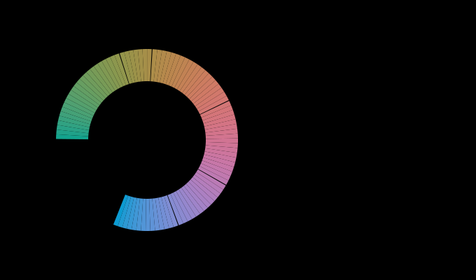
The purple and magenta region between blue and red is one quadrant of quadrature and two-fifths of the hue circle. That is a real perceptual statement — there is no unique purple, so the model has no anchor there and the interpolation stretches across the gap. It is also the region where the eleven basic colour terms are most crowded, which is the opposite arrangement and is worth noticing rather than reconciling.
What a tolerance in quadrature costs
The practical consequence follows directly and is the reason to have the numbers.
A hue tolerance stated in quadrature — within five units of H — is a tolerance in hue angle of 5 divided by the local slope. Near yellow that is 2.6 degrees. Near blue it is 10.7 degrees. The same stated tolerance is four times tighter at one hue than at another, measured in the quantity an instrument reports and a device drifts in.

The same applies to a hue-preserving gamut mapping. Preserving hue means holding one of the two scales fixed, and holding quadrature fixed is not holding the angle fixed — a mapping that walks a colour inward at constant H is walking it at a hue angle that changes, by a rate that depends on where it started — and no mapping preserves everything is the general form of that.
Which of the two a mapping preserves is a decision, and specifications say only hue-preserving. It joins the arrangement of a raw pipeline on the list of decisions nothing records. The difference between the two is bounded by the same factor of four, and it is largest exactly where the mapping has the most work to do, which is the saturated blues and purples.

That the two coincide is worth a sentence. The hues where the quadrature runs slowest are the hues where the inverse’s domain is tightest, and both are consequences of the model’s cone matrix having very unequal rows. One matrix produces both the boundary and the unevenness, which is why the two figures have the same shape and is not a coincidence to be explained away.
The two hue scales, and which one anybody means
A model that reports hue twice puts an obligation on whoever uses it, and the obligation is usually ignored.
A colour difference computed in CAM16-UCS uses the angle, because the UCS coordinates are built from the opponent signals directly. A hue tolerance in a specification is usually written in quadrature, because quadrature is the scale with names attached to it. A hue-preserving gamut mapping holds one of them fixed and the documentation rarely says which.
Those three are not the same operation, and the gap between them is bounded by the factor of four above and is largest in the blues and purples.
The cleanest statement is that quadrature is for describing and the angle is for computing. A person saying this is a slightly yellowish red means something about quadrature; a formula measuring how far apart two colours are is working in the angle. Using quadrature in a distance calculation imports its unevenness into a number that is supposed to be uniform, and using the angle in a description imports a zero point that means nothing.
The practical rule is to state which. It is one word in a specification and it is worth four times a hue tolerance’s own value.
What was computed, and how
The anchors and weights are the CIE’s own, as the model publishes them, and the interpolation is the standard’s formula implemented directly. Nothing here is a re-derivation: the slopes are finite differences of the published function at a step of a hundred-thousandth of a degree, which is far above the floating-point floor and far below the scale of anything the function does.

The quadrature is the one correlate with no viewing condition in it. Hue angle depends on the adaptation and therefore on the room, and the map from angle to quadrature does not — so everything in this essay is a property of the model’s table rather than of the situation, which is unusual for this family of figures and is why every panel here holds the situation fixed.
The quadrant spans are differences between the published anchor hues and are exact.

The two unevennesses are worth putting side by side because they are independent. Lightness runs unevenly because it is a compression with an exponent in it; hue quadrature runs unevenly because it is an interpolation through unevenly spaced anchors with unequal weights. Neither is a defect and both are invisible in the number. A specification quoting J to a tenth and H to a unit has quoted two requirements that each vary by a factor of several across the space they apply to, and has quoted them in the tone of a measurement.
What the corners are worth in practice
A corner in a scale is a small thing unless something differentiates it, and two things do.
An optimisation does. A gamut mapping, a fit, or any search that moves a colour to minimise a distance is following a gradient, and a gradient that jumps by a factor of 1.74 across a point is a gradient a solver can oscillate about. Nothing here has observed such an oscillation and the mechanism is standard: a piecewise-linear objective’s corners are where descent methods slow down or stick.
And a tolerance boundary does. Two colours straddling an anchor are being compared through two different local rates, so the answer to are these within five units of hue depends on which side of unique green they sit — not in the sense of being harder to compute, but in the sense that the same physical hue difference reads as two different numbers.
The four anchors are at hue angles 20, 90, 164 and 238, which are a red, a yellow, a green and a blue. Those are four of the most common colours anybody specifies, so the corners are not in a remote part of the space; they are exactly where the traffic is.
Where the model stops
The four anchors are measurements with uncertainty on them, and the uncertainty is not small: reported unique hue loci vary between studies by several degrees and between observers by a great deal more. The corners are therefore sharp in the model and not in anybody’s eye, and a scale fitted to a different set of unique hue data would have its corners in different places.
Nothing here says the interpolation is the wrong one. A smooth interpolation through the same four points — a spline, say — would have no corners and would not pass through the anchors with the right slopes either, since nothing measures those. The corner is the price of exactness at the nodes.
And the unevenness is a statement about the model’s own hue angle, which is not a perceptual quantity. Saying that quadrature runs four times faster in one place is saying that the model’s two hue scales disagree by that much about spacing; which of them is closer to what an observer would report is a question this collection has no data to answer.
The generalisation
The habit is about a quantity that is a table rather than a formula.
In a model built almost entirely of algebra, one quantity that is interpolated between measured anchors reads exactly like the others: same name, same units, same place in the output. Its behaviour is different in every way that matters — it is exact where the data are and constructed everywhere else, it is not smooth at the nodes, and its rate is whatever the node spacing makes it.
The move is to plot its derivative once. A corner is invisible in the function and unmistakable in the slope, and the plot takes a minute.
The failure mode is that the table’s quantity gets used as though it were uniform, because everything around it is. A tolerance quoted in an interpolated scale is quoted in units that vary, and nothing in the number says so — which is the same shape as the tolerance problem two ladders across and arrives from a completely different direction.
Who found it, and when
Hue quadrature dates from Hunt’s appearance models and the four-anchor form is essentially unchanged from CIECAM97s through CIECAM02 to CIECAM16. The anchor hues and their weights are published in the standard and the interpolation is stated there in full.
The unevenness is implicit in those published numbers — anybody can subtract 90 from 164.25 — and does not appear to be discussed as a property of the scale. The nearest thing in the literature is the recurring observation that CAM16-UCS is more uniform than its predecessors in the blue region, which is the same region and a different measurement.
Where the ladder goes next
Two rungs have now found that the model’s coordinates are less regular than they look. The next question is about the model’s nonlinearity rather than its coordinates, and it has a surprising answer: averaging the model’s predictions is very nearly averaging its argument, over the one argument this collection has spent a round measuring, and not at all over another.
Where this goes next
 Why there are four unique hues
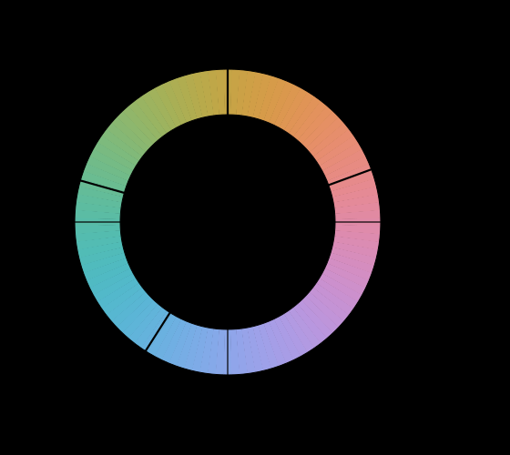
Observers agree that four hues are elementary and that no colour is reddish green. Nothing in the three receptors predicts either fact, and the axes of every standard colour space miss the four by tens of degrees.
Why there are four unique hues
Observers agree that four hues are elementary and that no colour is reddish green. Nothing in the three receptors predicts either fact, and the axes of every standard colour space miss the four by tens of degrees.
 An appearance is not always a stimulus
CIECAM16's inverse is a closed form that returns three numbers for every lightness, chroma and hue it is handed. Whether those three numbers are a light it does not ask, and over a lattice spanning the space a specification is written in, 10.8 per cent of them are not — one tristimulus value negative, or a relative luminance above the white's. Only 43.8 per cent are colours a display could show at all.
An appearance is not always a stimulus
CIECAM16's inverse is a closed form that returns three numbers for every lightness, chroma and hue it is handed. Whether those three numbers are a light it does not ask, and over a lattice spanning the space a specification is written in, 10.8 per cent of them are not — one tristimulus value negative, or a relative luminance above the white's. Only 43.8 per cent are colours a display could show at all.
 The straight piece under the cube root
CIELAB's lightness is described everywhere as a cube root and below a stated luminance it is a straight line, spliced on with two constants chosen so the join is exact in value and in slope. Every black a delivery chain reaches is inside that straight piece — a press black at L* 2.4, a projected black at 1.1 — where the compression does not compress, the price of a deviation is flat to two parts in a thousand, and the second derivative the composition of two departures needs does not exist.
The straight piece under the cube root
CIELAB's lightness is described everywhere as a cube root and below a stated luminance it is a straight line, spliced on with two constants chosen so the join is exact in value and in slope. Every black a delivery chain reaches is inside that straight piece — a press black at L* 2.4, a projected black at 1.1 — where the compression does not compress, the price of a deviation is flat to two parts in a thousand, and the second derivative the composition of two departures needs does not exist.
What this makes readable
Essays that name this one as a prerequisite.
Named alongside this one
Essays reaching for the same objects. Nobody chose these; they are what the index of named objects makes visible.
- A contrast control is three controls colour appearance · hue quadrature · specification · structural choice
- A stated lightness is two requirements ciecam16 · colour appearance · specification · tolerance
- A chain measured in a unit that cannot add ciecam16 · specification · structural choice
- A dark background moves every difference and no match ciecam16 · colour appearance · tolerance
- A dial has a price ciecam16 · interpolation · specification
- A display in a room is a smaller display ciecam16 · colour appearance · specification
What links here
Every essay whose body links to this one.
The objects this essay names
Each one links to every other essay that touches it.
AnisotropyCIECAM16Colour appearanceHue quadratureInterpolationNamingSpecificationStructural choiceToleranceUnique hues