The average surface does not look average

Averages are taken on both sides of an appearance model, and whether they commute with it decides whether an average can be carried through. Where the model’s curve does not matter asked the question over two arguments: over a population of observers, where the mean of the model’s predictions is its prediction for the mean to within 1.4 per cent of the spread, and over the range of light one room sees in a day, where the same gap is 59 per cent. It did not ask over surfaces, which is what a scene is made of.

A fifth of the spread #

Averaging surfaces does not commute with the appearance model: the average surface looks lighter than the surfaces do on average, by an amount that depends on how many dark surfaces the set contains.

• Over 240 smooth natural reflectances the gap is 20.8 per cent of the spread, fifteen times what it is over a population of observers.
• The mean surface’s lightness J′ is 77.0; the mean of the surfaces’ lightnesses is 72.8. Almost the whole gap is lightness.
• On a banded family with dark members the gap is 27.4 per cent and the lightness difference 7.3 units; on a pale family it is 9.2 per cent and 0.8.
• The grey with the average light is a 46.9 per cent reflectance; the grey with the average look is a 43.1 per cent one, and on the family with dark members 31.5 against 26.5.

Three spreads and one inequality #

The mechanism is the one that governs every average through a curve. The model’s lightness is a concave function of the stimulus — it compresses — and the average of a concave function’s values is below the function of the average. So the average of the surfaces’ lightnesses is below the lightness of their average surface, always, by Jensen’s inequality. What varies is the size, and the size is set by how far along the curve the inputs spread.

A population of observers moves a stimulus a very short way. Two people looking at the same surface differ by a colour difference or two, which on a curve spanning the whole range of lightness is almost a straight segment, and the inequality is there with a gap of 1.4 per cent of the spread. A room’s light over a day moves the adapting luminance across two decades, which is a long stretch of a curved function, and the gap is 59 per cent.

Surfaces are between the two. A scene contains surfaces from nearly black to nearly white, so the stimulus moves across most of the lightness range — further than observers move it — but it moves along the lightness axis of a curve whose bend is gentler than the adapting luminance’s fourth root. The gap lands at a fifth of the spread.

The bend times the spread #

The inequality fixes the sign, and a second-order expansion says what sets the size. For inputs spread a little around their mean, the average of a curve’s outputs falls below the output at the average by about half the curve’s bend there, times the variance of the inputs. A curve that bends twice as hard doubles the gap; inputs spread twice as far quadruple it.

Both factors are visible in the first figure’s row of spreads. Observers barely spread a stimulus, so the variance is tiny and the gap is 1.4 per cent. A day’s light spreads the adapting luminance across two decades of an argument the model compresses hard, so both factors are large. Surfaces spread lightness widely, and the lightness curve bends hardest near black — which is why the share of dark surfaces in a set, and not its size or its hues, is what moves the number. It is the same mechanism that makes a blend of stored values darker than a blend of the light: a concave function, a set of inputs, and an average taken on the wrong side of it.

The mean surface is lighter than the surfaces look #

The first figure reports a share. The quantity underneath it is a lightness, and it is easiest to see as two lines through one distribution.

The 240 reflectances run from dark to light with slopes and curvatures walked over a lattice, and their lightnesses spread across most of the scale. The mean of those lightnesses is 72.8. The mean reflectance, which under one lamp gives exactly the mean tristimulus value because the colour integral is linear, has a lightness of 77.0.

The vector gap in the model’s uniform space is 4.35 units, and 4.2 of them are lightness. The hue components nearly cancel because the average of many surfaces of many hues is nearly neutral either way. The inequality lives almost entirely on the axis the compression acts along.

Dark surfaces enlarge it #

The size of the gap depends on how much of the curve the set covers, and the steep part of the curve is at the dark end. A set with more dark surfaces in it has a larger gap.

The banded family at four reflectance levels reaches down to L* 18. Its gap is 27.4 per cent of the spread and its lightness difference 7.3 units — the mean of its lightnesses is 58.7 and the lightness of its mean surface 66.0.

The audit’s own forty-two surfaces sit at the other extreme. A mean has a set under it, and that set was chosen once with every surface pale: L* 57 to 93. On those surfaces the gap is 9.2 per cent of the spread and the lightness difference 0.8 units. A measurement made on the pale set would have found the average surface looks very nearly average, and it would have been a statement about paleness.

The second-order term says why. The pale set’s surfaces all sit on the upper stretch of the lightness curve, where it bends least, and they spread only from L* 57 to 93, so both factors of the gap are small at once. A set chosen to vary hue and band position while holding every surface pale is a set built, without meaning to be, to make an average look safe to carry through a nonlinearity, and every later average over it inherits that safety without inheriting its reason.

Two greys #

A lightness difference of four units is abstract. The same result stated as a pair of greys is not.

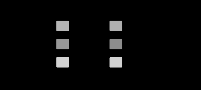
For the smooth set, the grey with the lightness of the average light is a 46.9 per cent reflectance, and the grey with the average lightness is 43.1 per cent. For the banded family with dark members the two greys are 31.5 and 26.5 per cent, a larger difference relative to either. For the pale set they are 65.3 and 64.4 — nearly the same grey.

Those are two answers to a question photographers ask every day: what grey is the middle of this scene? The first grey is the scene’s average light. The second is the scene’s average appearance. An exposure meter that averages luminance finds the first.

What it does to middle grey #

Middle grey is usually defined as an eighteen per cent reflectance, and the definition is justified two ways that are rarely distinguished. Eighteen per cent has a lightness of about 50 on CIELAB’s scale, so it looks halfway between black and white. And a scene’s average reflectance is said to be about eighteen per cent, so a meter calibrated to it exposes an average scene correctly.

The second justification is an average of light and the first is a statement about appearance. The result here says the two are different averages, and that the gap between them depends on the scene’s content: a scene with a few dark surfaces and many light ones has an average light that looks lighter than the scene does. A meter reading the average light of such a scene sets exposure for a grey lighter than the scene’s own middle.

That is not an argument against metering. It is a statement of what a meter measures, and the size of the difference — five points of reflectance on a scene of dark and light surfaces — is large enough to be one of the reasons experienced photographers correct a meter’s reading by eye.

A meter, a highlight and a viewer #

Two families of automatic exposure answer two different questions, and the two greys place both. An averaging meter takes a scene’s mean light and renders it as a fixed output grey, so it is tied to the first grey. A highlight-based exposure puts the brightest surface near the top of the output and lets everything else fall where it falls — the logic by which the highlight is the white balance in a converter. Neither is tied to the scene’s average appearance. A meter reads luminance, and brightness is not luminance; the grey a viewer would call the middle of the scene is the second grey, and no light meter measures it.

In stops the difference is modest. On the smooth set, 46.9 against 43.1 per cent is an eighth of a stop; on the set with dark members, 31.5 against 26.5 per cent is a quarter of a stop. A quarter of a stop is within the range of corrections photographers routinely apply to a meter reading, and its direction follows from the result: an averaging meter renders the scene’s perceived middle darker than middle grey, so the correction it calls for is a little more exposure, and more for a scene with deeper shadows in it.

The case where the two greys part most is not exotic. A scene of mostly pale surfaces with a few deep shadows — pale walls, a dark doorway, dark furniture — is the ordinary interior, and it is exactly the distribution the family with dark members approximates.

What it does to grey world #

A grey-world illuminant estimate assumes the average surface in a scene is neutral and reads the illuminant off the average stimulus. The algorithms that guess the light described the assumption and what violates it.

The result here leaves grey world’s chromaticity alone. The average of many surfaces is very nearly neutral in both senses — the mean surface’s colourfulness is 0.9 units, and the hue components of the mean appearance nearly cancel too. Grey world estimates the direction of the light from a chromaticity, and averaging stimuli and averaging appearances give nearly the same neutral direction.

What it changes is the lightness of the grey the scene is assumed to average to. A white-balance algorithm that also sets exposure from the scene’s average — as camera auto-exposure does — inherits the difference between the average light and the average look, and in a high-contrast scene it will be several units of lightness.

Colourfulness averages the other way #

One quantity behaves differently from the rest, and it is worth separating because it is easy to misread.

The mean surface is almost exactly neutral: its colourfulness M is 0.9. The average of the surfaces’ colourfulnesses is 11.4. Averaging the surfaces cancels their colour; averaging how colourful they look does not, because colourfulness is a magnitude and magnitudes do not cancel. That is not Jensen’s inequality — it would happen for a perfectly linear model — and it is the reason the first figure uses the vector mean in the model’s space, whose colourfulness is 1.4, rather than the mean of the magnitudes. A statement that a scene’s average colourfulness is eleven and a statement that its average colour is neutral are both true.

What it does to an average over a census #

The most direct consequence is for numbers that are averages of appearances over a set of surfaces.

An adaptation census reports the mean residual of a transform over a set of surfaces, and an appearance audit reports the mean of a departure’s cost over a set of surfaces. Neither mean is the residual or the cost of the mean surface, and the difference is a fifth of the spread on an ordinary set. The earlier licence to carry averages through the model covered observers, and this result says it does not extend to surfaces. A mean over surfaces has to be taken after the model, never before it, and it has to name its set.

What was computed, and how #

Each surface’s reflectance is multiplied by D65 and integrated through the 1931 observer to tristimulus values relative to the white, then read by CIECAM16 at an adapting luminance of 100 candelas a square metre, a twenty per cent background and an average surround. The appearances are taken to CAM16-UCS’s J′a′b′.

The mean appearance is the vector mean of J′a′b′ over the set. The mean surface’s appearance is the model’s reading of the mean tristimulus value, which is exactly the reading of the mean reflectance because the integral is linear. The gap is the Euclidean distance between the two, and the spread is the root-mean-square distance of the set’s appearances from their mean.

The greys are the neutral reflectances whose model lightness equals the two lightnesses being compared, found by inverting the model on the neutral axis.

Where the measurement stops #

The smooth set is a construction walked over a lattice of level, slope and curvature, and the banded family is a construction too. Neither is a measured scene. The gap depends on the distribution of lightness in the set, so a measured scene with a known distribution would give its own number, bracketed by the three here.

The model is read under one lamp in one room, with every surface adapted to the same white, as though each were a patch in a fixed surround — and a patch is not a scene. A real scene has illumination varying across it and a viewer whose adaptation is local, and both would change which average is the relevant one.

And the model’s lightness is a model. The inequality is certain for any compressive lightness scale; its size belongs to CIECAM16’s compression and would differ for CIELAB’s.

The habit #

The habit is about the order of an average and a nonlinearity.

Whenever a set of inputs passes through a curve, there are two averages available — of the inputs, then through the curve, or through the curve, then of the outputs — and they differ by an amount set by the curve’s bend times the spread of the inputs. The difference has a sign that a concave curve fixes.

The move is to ask how far the inputs spread along the curve before choosing which average to report. A spread of observers is short and the order barely matters; a spread of surfaces is long and it does.

The failure mode is to compute the easier average — usually the one of the inputs, because it is one call — and report it as the other. The appearance of the average is not the average appearance, and on a scene with dark surfaces in it the difference is a visible grey.

Who noticed it first #

Jensen’s inequality is from 1906 and its consequences for averages through compressive scales are standard in psychophysics. The distinction between a scene’s average reflectance and its perceived middle is part of photographic practice, usually expressed as the advice that a meter is calibrated to a grey rather than to a scene.

That the appearance model’s answer for the mean surface differs from its mean answer by a fifth of the spread on a smooth set, and by more on a set with dark surfaces, is measured here; the sources consulted here state the inequality and not its size.

Still open: the gap over a measured scene #

The number that would settle how much this matters in practice is the gap over the surfaces of a real scene, weighted by the area each occupies. That needs a scene with spectral reflectance and area for each surface — a hyperspectral image of an ordinary interior — and it would say whether a scene’s average light and its average look differ by the two points of reflectance a pale scene shows or the five a contrasty one does.