Theme

The thread: The instrument is the reader — page 5

This is the one subject where the page is displayed on the apparatus under discussion, and the reader's own eye is the measuring device. Several figures here are experiments rather than illustrations.
The dyes a camera has, and the dyes an adaptation basis would want. Three sensor sensitivities drawn twice: faintly, the silicon-and-filter-array set this collection models, and boldly, three Gaussian dyes chosen to make the inverse of their own response matrix a good basis for a white-balance gain. The designed dyes sit at 610, 542, 449 nm with widths of 35, 26, 30 nm — narrower and further apart than the real ones, which is what sharpening looks like when a search rather than a committee does it. They leave 0.97 ΔE00 against the real sensor's 1.62, and they are held within 0.28 of the Luther condition so that the result is still a camera. What a camera does

A sensor designed for its inverse

A camera's white balance is a gain in a basis made from its own dyes and the light in the room. Choose the dyes for that basis instead of for cost and quantum efficiency, hold the sensor within a stated distance of the Luther condition, and the design reaches the best adaptation figure any basis achieves — and then the room moves it.

Four cameras that all satisfy the Luther condition exactly. Four sensors whose sensitivities are linear combinations of the colour-matching functions — the theoretical ideal, satisfying the condition to machine precision, each with an adaptation basis that does not move when the light does. They differ only in which linear combination, which the condition does not constrain, and they leave 2.46, 0.97, 1.65, 2.37 ΔE00 after a white balance. The best of them reaches 0.974, which is the best any basis at all achieves. Being a perfect colorimeter costs nothing in adaptation; what costs is the mixing matrix, and the control measured here carries one nobody chose. What a camera does

The condition chooses no axes

It has long been said here that a sensor satisfying the Luther condition exactly adapts worse than a silicon one, and offered a reason — that its channels are the matching functions, and a gain on those is the oldest mistake in the subject. The measurement was of one sensor. The condition leaves the axes entirely free.
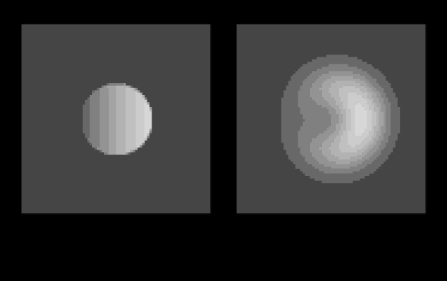
The same border signal, filled in with a boundary and without one. Two fields, each 6 degrees across. The signal is injected along a ring just inside a contour and varies around it, brightest on one side and dimmest on the other. On the left the signal diffuses and the contour is impermeable: the interior settles to 1.000 against a border mean of 1.000, which is the mean-value property of a harmonic function arriving as a prediction about appearance. On the right the same signal is handed to a Gaussian pool of 0.5°, which has no notion of inside: it reaches 0.040 at the centre, because a kernel weights the near rim more than the far one and a filled region does not. What a scene does

A pool with an edge

A Gaussian pool says how much of a stabilised image survives and can say nothing about what the remainder looks like, because a Gaussian has no edge. Give the pool a boundary and the interior of a faded region takes the average of its own border — exactly, by the mean value theorem, arriving as a prediction about appearance.

A gap in the wall and a gap in the drive are not the same gap. What the centre of a region settles to under three conditions. With the contour closed it reaches its border's value exactly. Open a 16% hole in the barrier and leave the border signal unbroken and it still reaches it, to 1e-8 — a ring of driven cells encloses the centre whatever the wall outside it is doing, so nothing can escape. Break the signal too and it falls to 0.960. All of what a gap costs is the piece of border that stopped driving, and none of it is the hole. What a scene does

A gap in the drive, not in the wall

Break the contour around a region and leave its border signal unbroken, and the interior does not move by one part in a million — a ring of driven cells encloses a centre whatever the wall outside it is doing. Break the signal too and the shortfall goes as the square of what is missing. All of what a gap costs is the piece of border that stopped driving.

The same optimum, along its narrowest direction and its widest. The adaptation objective along two straight lines through its own minimum, both of unit length in the nine coefficients. Along one of them the cost rises steeply; along the other the same step costs 8.0 times less, and a design constrained to move that way gives up almost nothing. That is why restricting the nine numbers to be the inverse of three realisable primaries — three degrees of freedom gone — costs about one per cent, while requiring them to hit the three dichromat confusion points costs seventy. Counting what a constraint removes predicts neither number; what matters is which way it points. Where the model breaks

A constraint costs what it points at

Three primary chromaticities remove three of the nine numbers in an adaptation basis and cost one per cent. Three dichromat confusion points remove six and cost seventy. Counting what a constraint removes predicts neither, because an optimum is a long bowl and what matters is which way the constraint points.

The points a ratio needs are proportional to the ratio. A scatter of 133 points on logarithmic axes, one per MacAdam ellipse under each of six coordinate systems. The horizontal position is that ellipse's true axis ratio; the vertical is the smallest sample size, from a sequence of doublings, at which the sampled ratio comes within one per cent and stays there. A line of slope 0.94 runs through them, against a predicted 1 — the minimum's notch is 0.88 σ₂/σ₁ radians wide, so resolving it takes a number of points proportional to σ₁/σ₂, and nothing about the basis or the ellipse enters beyond that. An ellipse with a ratio of two needs seventeen points and one with a ratio of twenty-six needs a hundred and ninety-two. Where the model breaks

An extremum is not a sample

Three separate measurements in this collection took a maximum or a minimum over a sample of a set — forty-eight points round an ellipse, twenty-four directions out of an optimum, fourteen changes of light off a list. All three are wrong, all three are wrong in the same direction, and the error in each grows with the very quantity being measured.

A template that cannot place a point, fitted three ways. Three rows, one per set of stimuli the pigment template's cone matrix can be fitted over, each listing the three confusion points that matrix implies. The protanope's point wanders from (0.99, 0.20) to (0.76, 0.13) against a measured (0.75, 0.25), and the deuteranope's moves by 22.5 in chromaticity — further than the whole diagram is wide. A copunctal point is where two nearly parallel planes meet, so a template good to a few per cent, which is far more than enough to place a spectrum, is nowhere near enough to place this. It is why the population is built by moving the measured points rather than by deriving them. What the eye does

A template cannot place a point

This collection's model of an eye is good to a few tenths of a per cent at predicting what a cone catches, which is far more than enough to place a spectrum. Asked where that eye's confusion points are, it puts the protanope's at (0.99, 0.20) against a measured (0.75, 0.25) and the deuteranope's anywhere from (1.1, −0.5) to (−18, 11) depending on which stimuli the fit was made over.

Every width at the wide end of its span, and at the narrow end. One line per published quantity, each spanning the value it takes when all four declared widths are read at the narrow end of their reported ranges to the value at the wide end, with a marker at the value as declared. The largest span is the deutan margin at a factor of 2.62; the smallest is 1.22. This is the reading the population model's own documentation promised for four phases and nothing ever took. It is not a confidence interval — the four ends are not quantiles and the widths are not independent draws — it is what a reader who distrusts all four at once sees. What the eye does

A width nobody varied

Five numbers say how much people differ from one another, and every conclusion drawn here about a population rests on them. Each was written down with the range the literature reports beside it, so that a result could be re-read at the pessimistic end. Nothing ever was.

Which width carries the answer, and which carries the doubt. Two columns of bars over the four things that differ between two pairs of eyes. On the left, the share of the population's disagreement each one accounts for — the attribution quoted here since the population was built, which puts the lens first at 81%. On the right, how much of the doubt each one puts on everything published here, which is its elasticity multiplied by how badly the width itself is known. The macular pigment comes first there, at 0.65 against the lens's 0.60 — a lead of 8%. The two lists agree exactly below the top. What the eye does

Which measurement is worth making

Four things about an eye differ between people, and they have been ranked here by how much of the answers they carry since the population was built. Ranking them by how much doubt they carry gives a different order, and ranking them by which one takes a published claim closest to failing gives a third.

How wrong the ellipses would have to be for a pair to change places. One bar per adjacent pair in the uniformity table: the relative error on each ellipse's own axes at which that pair changes places in one draw in twenty. No error on the data is quoted anywhere — the question is inverted, so what is reported is how large an error would have to be, and a reader with an opinion about MacAdam's experiment can compare it with their own number. The nearest pair goes at 0.171; 2 of the 7 pairs do not reverse under any error this search covers. Difference and uniformity

How wrong would the data have to be

Twenty-five ellipses measured on one observer in 1942 are the ruler every colour space here is judged against, and they have never been given an error. Rather than invent one, the question is turned round, and asks how large an error would have to be before the ranking changed.

Twenty-five ellipses is a sample, and the score has an error bar. One row per colour space this collection ranks: the mean axis ratio its ellipses come out at, with the standard error of that mean over the twenty-five ellipses it was computed from. No literature is quoted — a mean of twenty-five numbers has a standard error those twenty-five numbers determine. The bars are far from equal: the best space carries ± 0.07 and the worst ± 1.56, because a space that makes the ellipses nearly circular makes all of them nearly circular and one that does not is dominated by whichever ellipse it handles worst. Difference and uniformity

Twenty-five is a sample of the diagram

A colour space's uniformity score is the mean of twenty-five numbers, and a mean of twenty-five numbers has a standard error those twenty-five numbers determine. Nothing has to be quoted to compute it, and three of the seven adjacent pairs in this collection's ranking survive it.

A mid-grey's lightness across a continuum of rooms. The lightness a mid-grey is predicted to have, plotted along the continuous surround parameter running from an average room to a dark one. The three rooms the standard tabulates are marked on it: average at the left, dark at the right, and dim 61% of the way between them rather than halfway. The whole span is 9.71 units of lightness and the step from average to dim is 5.64 of it — 58% — so choosing one of the three rows is a decision worth most of the range. What the brain does

The surround is three rows of a table

An appearance model takes the room as three constants, and the standard tabulates three rooms. Every appearance figure in this collection is drawn at one of them. The parameter they are three points of is continuous, and the middle row is not in the middle.

Every adaptation number here assumes a complete adaptation. Three curves and their mean: the colour difference an adapted observer is left with after a change of light, against the degree of adaptation from zero — no adaptation at all — to one. Every adaptation figure in this collection is computed at one, the right-hand end. The appearance model's own formula puts the degree at 0.941 for an average surround at a hundred candelas, marked, where the residual is 2.21 ΔE00 rather than 1.27 — larger by a factor of 1.74. The left-hand end is exactly the unadapted change, which is not an approximation but an identity, and is what says the curve interpolates between the two things it claims to. What the brain does

A discount nobody measured

Every adaptation number in this collection assumes an observer who adapts completely. The appearance model's own formula says they do not — it puts the degree at 0.94 in an ordinary room — and the difference is not a rounding. It is a factor of 1.7 on the residual every one of those figures reports.

A quadratic is believed least far at the one place anybody takes one. One bar per basis: the radius, in the nine coefficients, within which the second-order model predicts the objective to within ten per cent in every one of eighteen directions. The shortest bar is the objective's own optimum, at 2.3×10⁻², and the longest is XYZ scaling at 1.1×10⁻¹ — several times further. The reason is not that the model is worse at a minimum but that it has less to do there: away from one the linear term is exact and carries most of the change, so a ten per cent error in the prediction takes longer to accumulate. It does not make a Hessian at a minimum wrong; it says the picture drawn from it describes the smallest neighbourhood in the table. Where the model breaks

How far a quadratic can be believed

A second-order model has a radius inside which it describes a surface and outside which it does not, and that radius can be measured. Measured at eight places on one objective, it is smallest at the optimum — the one place anybody ever takes a Hessian.

Room is not safety: two orderings of the same three claims. Three pairs of bars, one pair per published statement about the confusion points. The upper bar in each pair is the margin — how far the measured number is from the threshold that makes the statement true, as a ratio. The lower bar is the headroom — the factor by which one declared width of the population model would have to be wrong for the statement to fail. Both start at one, which is the line. Ordered by margin the three read the protan margin, the tritan margin, the deutan margin; ordered by headroom they read the protan margin, the deutan margin, the tritan margin, and the middle two change places. Every one of the three is inside a factor of two of failing, which the margins do not say. Where the model breaks

What would have to be wrong

A great many statements here have thresholds written into them, which turns out to make an audit possible — for each one, the smallest change in a declared input that would stop it holding. Most are unreachable. One is inside a factor of one and a third.

The winner survives the census's own construction; the middle of it does not. One row per perturbation of a constant the adaptation census is built from — the imaginary wall's centre wavelength, its width, its depth, its base, the macular filter's density and the two lens ages — each moved by an amount plausible for that quantity in its own units, up and down, and then all of them together. Each row shows where the five published transforms rank under it. Bradford holds the first column in all 14 rows. The second and third columns, which the table as built separates by six parts in a thousand, change places in 2 of them — so that ordering was never a fact about the transforms. What light is

The census is a construction too

Five of the fourteen changes of light this collection scores adaptation transforms against are not measurements of anything — they are a wall somebody invented, at a wavelength somebody chose. Moving those constants by amounts plausible in their own units moves the mean residual by two fifths and never changes which transform wins.

A camera's dye widths are free under one requirement and not under another. Three panels, one per dye. In each, a pair of bars per requirement: how far that dye's centre wavelength and its bandwidth can move before the requirement gets five per cent worse. Under the adaptation objective — the one the previous round measured — every width has far more room than its centre, which is the finding that put a tolerance budget on the centres. Throughput and the colour matrix's noise gain, the two requirements that objective was said to be silent about, reach the edge of the search in every direction and hold nothing. What tightens the widths is the Luther residual, which was in the model already. The bottom pair in each panel is what survives all four. What a camera does

The widths were free because nothing else was asked

A camera's three dye bandwidths carry almost all of the flattest direction of the adaptation objective, so that objective says a tolerance budget belongs on the centre wavelengths. The two requirements it was said to be silent about turn out not to bind either — and the one that does was in the model already.

Exactly flat everywhere, and eigenvectors at one point only. Two columns over the same nine places. On the left, how far from zero the objective's second derivative is along a row-scaling direction, on a logarithmic axis — it is between 10⁻⁹ and 10⁻⁶ of the largest eigenvalue at every one of them, which is a numerical zero. Scaling a row of the basis is a straight line along which the cost does not change, and that is true at every point, not only at the optimum. On the right, the angle between those three directions and the Hessian's own three smallest eigenvectors: 0.025 degrees at the optimum and up to 88 away from it. An invariance is a property of the function; being an eigenvector is a property of the function at a minimum, and the two coincide only where everybody computes. Matching and measuring

Only the flat directions keep their names

Three of the nine numbers a colour match leaves free do nothing, and they do nothing everywhere — exactly, at every basis in this collection's table. They are the objective's own principal directions at one point only, and everywhere else the directions carrying the curvature have turned by tens of degrees.

At a published matrix the slope arrives long before the bowl. One row per basis in this collection's table. Each row is a logarithmic axis of distance in the nine coefficients, with two markers: the radius at which the objective's curvature becomes as large as its slope, and the distance from that basis to the optimum. The first is between 3.2 and 108 per cent of the second. So over almost the whole journey from a published matrix to the best one, the surface is a slope and not a bowl — and a table of eigenvalues taken there describes a neighbourhood the optimum is nowhere near. XYZ scaling is the exception, at 1.08 of the distance, because its slope is the steepest in the table. What it takes to deliver it

The slope arrives before the bowl

The adaptation transforms colour management actually uses are not optima of anything. At every one of them the objective has a slope, and the slope is the larger term over almost the whole distance to the best matrix — so a table of curvatures taken there describes a bowl nobody meets on the way anywhere.

Downhill from every published matrix, one step at a time. Each curve is a steepest-descent walk from one of this collection's published bases, plotted as the objective against the distance walked in the nine coefficients. The horizontal line is the optimum. The first step of each walk is the long one — XYZ scaling closes 41 per cent of its whole gap in one — and every walk then flattens without reaching the line, because the valley floor is nearly flat and the steepest direction is nearly across it. Bradford starts closest and closes least: it is already in the flat part. What it takes to deliver it

Downhill from a published matrix

Walking steepest descent from each adaptation transform in use closes between a quarter and nine tenths of its distance to the best one, and most of that in the first step. The direction it sets off in is eighty to eighty-seven degrees away from the answer, and that turns out not to be an artefact of the three directions nothing can see.

What one change of light costs, surface by surface — daylight to tungsten. A rising curve of 125 points, one per surface in the test set, sorted from the surface this change of light costs least to the one it costs most, with the published mean drawn across it as a horizontal line. The published residual for daylight to tungsten is 1.635 ΔE₀₀. The curve runs from 4.4e-14 — 5 of the surfaces are flat greys, on which an adapted observer's gain is exactly right and the residual is exactly zero — to 3.058, which is 1.87 times the mean. The mean line crosses the curve about two thirds of the way along, so most surfaces cost less than the published number and a minority cost a great deal more. This is what a single published residual is a summary of. What a scene does

A mean has a set under it

Every adaptation number this collection publishes is an average over a hundred and twenty-five surfaces that were written down once, in one file, with no argument for how many there should be or how saturated. The average runs from exactly zero to twice itself across them, and the set has never been varied.

Every census row under five constructions of the same test set. A slope chart with 5 columns — lattice, coarse, fine, uniform, natural — and one line per change of light in the census, each line joining that row's mean residual under each construction. Four of the five columns describe the same region of surfaces walked at different densities or against different measures; the last is the clamped, realistic family, which is not linear in its parameters and is therefore answering a slightly different question. The levels move: between the coarse and fine lattices every row shifts by seven to nine per cent, in the same direction, which is a common-mode factor no published residual here has ever carried. The order almost survives. Inside the region exactly one pair crosses, and it is the pair the standard error had already flagged; under the clamped set two more cross, including one the error separates by nearly nine standard errors. The crossing lines are drawn heavy. Difference and uniformity

A lattice is a quadrature rule

Walking a set of test surfaces more finely does not converge on a better answer, because refining a lattice under a constraint changes which corners of the region get sampled and not only how densely. The lattice used here turns out to be a two per cent biased estimate of the integral it stands for.

The error on a gap is not the two rows' errors added. Two bars for each of the 13 adjacent pairs in the census ranking. The upper, shorter bar is the standard error of the gap taken as a paired difference — the same 125 surfaces score both rows, so a surface that is awkward under one change of light is usually awkward under the other and the difference is quieter than either. The lower bar is the two rows' own errors added in quadrature, which is what comparing error bars by eye amounts to. Pairing is worth a factor of 1.78 on average and 3.36 on the pair it helps most, and it is the difference between 6 adjacencies unordered and 4. The gain is largest where the two rows are two daylights or two tungstens, because then the surfaces they find awkward are nearly the same surfaces. Difference and uniformity

The error on a gap is not the errors at its ends

Comparing two rows of a table by looking at whether their error bars overlap is the wrong comparison, and here it is wrong by a factor of up to 3.4. The same 125 surfaces score both rows, so the difference between them is quieter than either — and how much quieter is a measurement of how alike the two rows are.

Which steps of the census ranking the test set actually resolves. A horizontal bar for each of the 13 adjacent pairs in the census's ranking, from the smallest mean residual to the largest. A bar's length is the gap between the two rows in ΔE₀₀; the whisker on its end is twice the standard error of that gap, computed as a paired difference because the same 125 surfaces score both rows. Where the whisker reaches back past zero the pair is not ordered by this test set, and 4 of the 13 are in that state — marked. The largest steps, at the two ends of the ranking, are twenty standard errors wide and are not in doubt at all. The smallest is four parts in ten thousand between two rows the table prints as different numbers. What light is

Four steps the test set cannot order

The adaptation census prints fourteen numbers to four figures and its ranking is asked to say which lamps adaptation handles worst. Nine of its thirteen steps are established beyond any doubt the test set can raise; the other four are not, and three of them are consecutive — a tungsten lamp, a halogen lamp and a white LED are simply not ordered.

258 essays on this thread, page 5 of 11 · all threads · all essays