Theme

The thread: Computed, not quoted — page 11

Every swatch begins as a spectral power distribution and is carried through the colour-matching functions as it is drawn. None is a hex code recalled from a table.
What one change of light costs, surface by surface — daylight to tungsten. A rising curve of 125 points, one per surface in the test set, sorted from the surface this change of light costs least to the one it costs most, with the published mean drawn across it as a horizontal line. The published residual for daylight to tungsten is 1.635 ΔE₀₀. The curve runs from 4.4e-14 — 5 of the surfaces are flat greys, on which an adapted observer's gain is exactly right and the residual is exactly zero — to 3.058, which is 1.87 times the mean. The mean line crosses the curve about two thirds of the way along, so most surfaces cost less than the published number and a minority cost a great deal more. This is what a single published residual is a summary of. What a scene does

A mean has a set under it

Every adaptation number this collection publishes is an average over a hundred and twenty-five surfaces that were written down once, in one file, with no argument for how many there should be or how saturated. The average runs from exactly zero to twice itself across them, and the set has never been varied.

Every census row under five constructions of the same test set. A slope chart with 5 columns — lattice, coarse, fine, uniform, natural — and one line per change of light in the census, each line joining that row's mean residual under each construction. Four of the five columns describe the same region of surfaces walked at different densities or against different measures; the last is the clamped, realistic family, which is not linear in its parameters and is therefore answering a slightly different question. The levels move: between the coarse and fine lattices every row shifts by seven to nine per cent, in the same direction, which is a common-mode factor no published residual here has ever carried. The order almost survives. Inside the region exactly one pair crosses, and it is the pair the standard error had already flagged; under the clamped set two more cross, including one the error separates by nearly nine standard errors. The crossing lines are drawn heavy. Difference and uniformity

A lattice is a quadrature rule

Walking a set of test surfaces more finely does not converge on a better answer, because refining a lattice under a constraint changes which corners of the region get sampled and not only how densely. The lattice used here turns out to be a two per cent biased estimate of the integral it stands for.

The error on a gap is not the two rows' errors added. Two bars for each of the 13 adjacent pairs in the census ranking. The upper, shorter bar is the standard error of the gap taken as a paired difference — the same 125 surfaces score both rows, so a surface that is awkward under one change of light is usually awkward under the other and the difference is quieter than either. The lower bar is the two rows' own errors added in quadrature, which is what comparing error bars by eye amounts to. Pairing is worth a factor of 1.78 on average and 3.36 on the pair it helps most, and it is the difference between 6 adjacencies unordered and 4. The gain is largest where the two rows are two daylights or two tungstens, because then the surfaces they find awkward are nearly the same surfaces. Difference and uniformity

The error on a gap is not the errors at its ends

Comparing two rows of a table by looking at whether their error bars overlap is the wrong comparison, and here it is wrong by a factor of up to 3.4. The same 125 surfaces score both rows, so the difference between them is quieter than either — and how much quieter is a measurement of how alike the two rows are.

Which steps of the census ranking the test set actually resolves. A horizontal bar for each of the 13 adjacent pairs in the census's ranking, from the smallest mean residual to the largest. A bar's length is the gap between the two rows in ΔE₀₀; the whisker on its end is twice the standard error of that gap, computed as a paired difference because the same 125 surfaces score both rows. Where the whisker reaches back past zero the pair is not ordered by this test set, and 4 of the 13 are in that state — marked. The largest steps, at the two ends of the ranking, are twenty standard errors wide and are not in doubt at all. The smallest is four parts in ten thousand between two rows the table prints as different numbers. What light is

Four steps the test set cannot order

The adaptation census prints fourteen numbers to four figures and its ranking is asked to say which lamps adaptation handles worst. Nine of its thirteen steps are established beyond any doubt the test set can raise; the other four are not, and three of them are consecutive — a tungsten lamp, a halogen lamp and a white LED are simply not ordered.

Every census row under five constructions of the same test set. A slope chart with 5 columns — lattice, coarse, fine, uniform, natural — and one line per change of light in the census, each line joining that row's mean residual under each construction. Four of the five columns describe the same region of surfaces walked at different densities or against different measures; the last is the clamped, realistic family, which is not linear in its parameters and is therefore answering a slightly different question. The levels move: between the coarse and fine lattices every row shifts by seven to nine per cent, in the same direction, which is a common-mode factor no published residual here has ever carried. The order almost survives. Inside the region exactly one pair crosses, and it is the pair the standard error had already flagged; under the clamped set two more cross, including one the error separates by nearly nine standard errors. The crossing lines are drawn heavy. Where the model breaks

The instrument named the pair that moved

A standard error over a test set flagged four steps of the adaptation census as unresolved. Rebuilding the set three different ways reversed exactly one pair, and it was one of the four. Rebuilding it to a different rule reversed a pair the error separated by nearly nine standard errors — which is not a failure of the instrument but a statement of what it is about.

What a fourth reflectance dimension costs the theorem that a change of light is a matrix. Four rising curves on axes of the fourth dimension's amplitude, left to right, against what is left of daylight to tungsten after the exact 3×3 change-of-light matrix has been applied, in ΔE₀₀. All four begin at exactly zero: on the three-dimensional family the matrix is solved rather than fitted and there is no remainder at all, which is the theorem this collection's adaptation argument is built on. Adding a fourth reflectance dimension breaks it, and how badly depends far more on the fourth function's shape than on its size — at five per cent amplitude the four shapes cost 0.329, 0.572, 0.063, 0.124 ΔE₀₀ respectively, a factor of 9.1 between the dearest and the cheapest. For scale, the smallest von Kries residual anywhere in the census is 0.26 ΔE₀₀, so the cheapest of the four is a quarter of it and the dearest is twice it. What a scene does

A theorem about a family

A change of light acts on the test surfaces used here as an exact 3×3 matrix with no residual whatsoever, and the whole adaptation argument is built on that being exact. It is exact because the surfaces span exactly three dimensions, and they span exactly three dimensions because three basis functions were written down.

Which fourth dimensions are expensive, and how fine is too fine to matter. Two curves on axes of how many half-cycles a cosine fourth basis function makes across the visible band, against what it costs the matrix theorem in ΔE₀₀, at a fixed ten per cent amplitude. Both curves touch zero at exactly one and two half-cycles: those are the family's own second and third basis functions, so a fourth coefficient along them adds no dimension and a change of light stays exactly a matrix. Between them the cost climbs, reaches a maximum, and — for the smooth source — falls away again, because structure finer than the scale on which three broad cone sensitivities differ integrates to nearly nothing. The two curves part company at the fine end. Under daylight-to-tungsten the cost has fallen by a factor of 2.2 from its peak; under daylight-to-a-triphosphor-tube it has barely fallen at all, because a source with three narrow emission lines has structure of its own at that scale for the surface's structure to beat against. The observer is identical in both curves. What light is

A fourth dimension has a shape

How much a fourth reflectance dimension costs spans a factor of nine across four equally plausible shapes at one amplitude, and the expensive ones are not the shapes a variance figure would identify. The band that hurts is set by the illuminant rather than by the eye, which is why a triphosphor tube and a tungsten lamp disagree about it.

The census as the surfaces stop being three-dimensional. A slope chart with three columns — a test set with no fourth reflectance dimension, one with a fourth dimension at ten per cent amplitude, and one at twenty — and a line per change of light. Almost every line rises: a surface with structure the observer's three channels cannot follow is a surface an adaptation gain handles worse. Two lines are drawn heavy. daylight to a three-primary display rises fastest, by 90 per cent, because a source made of three narrow lines is precisely the instrument that cannot see a fourth reflectance dimension. And daylight to a triphosphor tube falls — the only row that does — because a triphosphor tube already samples the spectrum at three places, so extra structure in the surface is partly averaged away rather than added. The order of the middle of the table is not the same at the two ends; the extremes do not move. What light is

The row a fourth dimension improves

Giving the test surfaces one more degree of freedom makes almost every change of light harder for an adapted observer — but not all of them, and which one it helps depends entirely on what the extra dimension looks like. A triphosphor tube is improved by one shape and hurt more than anything else in the census by another.

How far each census row moves when the test set's own description does. A grid of bars, one row per change of light in the census and one bar in each row per number that describes the region the test surfaces are drawn from: how saturated they are, how bright, and how far the two modulations may go together. A bar's length is the elasticity — the proportional change in the published residual for a proportional change in that number. Saturation runs from 0.49 to 0.91 and brightness averages 0.104, so a test set's chroma range is nearly everything and its lightness range is nearly nothing. For scale, the largest elasticity found anywhere among this collection's five declared population widths is about a half — and those at least have declared ranges, while these three numbers have never been quoted with one. Difference and uniformity

Saturation is nearly everything

The set of test surfaces has three numbers describing it, and only one of them matters. How saturated the surfaces are carries an elasticity of about 0.7 on every result computed over them; how bright they are carries 0.10. A test chart's chroma range decides its answer and its lightness range does not.

How far each census row moves when the test set's own description does. A grid of bars, one row per change of light in the census and one bar in each row per number that describes the region the test surfaces are drawn from: how saturated they are, how bright, and how far the two modulations may go together. A bar's length is the elasticity — the proportional change in the published residual for a proportional change in that number. Saturation runs from 0.49 to 0.91 and brightness averages 0.104, so a test set's chroma range is nearly everything and its lightness range is nearly nothing. For scale, the largest elasticity found anywhere among this collection's five declared population widths is about a half — and those at least have declared ranges, while these three numbers have never been quoted with one. Where the model breaks

The input nobody declared

An audit that swept every declared width in this collection found the largest elasticity anywhere to be about a half. The most elastic input turns out to be one that was never declared, never quoted with a range and never varied — and being undeclared is exactly why it escaped the audit that was looking for it.

No one surface carries the answer, and the set is smaller than it looks. A falling bar chart of the 125 surfaces in the test set, ordered by how much each contributes to the published mean for daylight to tungsten. The tallest bar is 1.50 per cent of the total, so the mean is not a few awkward objects with a crowd behind them and a leave-one-out would move it by well under a per cent. The tail is the other half of the story: 5 surfaces contribute essentially nothing, because a flat grey is a surface an adaptation gain handles exactly. Counting the set by how evenly it contributes rather than by how many members it has gives 108.5 effective surfaces out of 125, which is what "a mean over a hundred and twenty-five surfaces" is really worth. What the eye does

The surfaces that answer nothing

Five of the hundred and twenty-five test surfaces contribute exactly zero to every number the adaptation census reports — not approximately, exactly — and the reason is the one fact about von Kries adaptation that makes it worth having at all. Counting the set by how much it contributes gives about a hundred members rather than a hundred and twenty-five.

A published residual is a mean, and the worst object in the room costs twice it. Three bars for each of the 14 changes of light in the adaptation census, ordered by how uneven the change is across surfaces. The first bar is the published mean residual. The second is the worst single surface in the audit's published test set. The third is the worst surface anywhere in the region that set is drawn from, found by search rather than by reading a maximum off a lattice. The mean-to-worst ratio runs from 1.90 to 4.02 and averages 2.43, so every published adaptation number has a worst case about twice it that no essay had ever quoted. The gap between the second and third bars is the other finding: a maximum over 125 sampled points understates the region's own maximum by up to 34 per cent. Where the model breaks

A mean is not a worst case

Every adaptation number this collection publishes is an average over objects, and the reader asking whether adaptation will fail them is asking about the object it fails on. That object costs between 1.9 and 4.0 times the published figure, and how uneven a change of light is across objects turns out to be a property of the change rather than a constant.

A published residual is a mean, and the worst object in the room costs twice it. Three bars for each of the 14 changes of light in the adaptation census, ordered by how uneven the change is across surfaces. The first bar is the published mean residual. The second is the worst single surface in the audit's published test set. The third is the worst surface anywhere in the region that set is drawn from, found by search rather than by reading a maximum off a lattice. The mean-to-worst ratio runs from 1.90 to 4.02 and averages 2.43, so every published adaptation number has a worst case about twice it that no essay had ever quoted. The gap between the second and third bars is the other finding: a maximum over 125 sampled points understates the region's own maximum by up to 34 per cent. Matching and measuring

An extremum is still not a sample

Two rounds ago three measurements turned up that took a maximum over a sample of a set and were short by up to a factor of two. The same error was live in a fourth place the whole time, on the set of surfaces every adaptation number is averaged over, and it is short by up to a third.

Every worst surface sits on a number somebody typed. The region the test surfaces are drawn from, in its own two modulation coordinates: a square of allowed depths with a diamond inscribed in it, the diamond being the requirement that the two depths sum to no more than 0.7. The 14 marked points are the worst surface for each change of light in the adaptation census, found by search over the whole region. Every one of them lies exactly on the diamond, and every one is also at the brightest level the region allows — both declared constraints active, on all 14 rows, with no interior maximum anywhere. That is the opposite of what bounding the wall gave: there the worst case turned over at a band width of six nanometres because a narrow band returns too little light, which is physics. Here the worst case is a reading of two numbers. The one constraint that is about the world — a paint's excitation purity may not exceed 0.6 — is slack everywhere: the most saturated surface the region admits reaches 0.459. What a scene does

Every worst surface sits on a declaration

Bounding the wall in a painted room produced a real worst case — the residual turns over at a band six nanometres wide because a narrower band returns too little light. Bounding the surfaces the residual is averaged over produces nothing of the kind, because all fourteen answers sit exactly on two numbers somebody typed and the one constraint that comes from the world never binds at all.

A confusion point is about the pigments that remain. Three groups of three bars. Each group is one dichromat's confusion point; each bar is how far that point moves in chromaticity when one of the three cone pigments has its absorption peak shifted by eight nanometres. In every group the bar for the pigment that dichromat is missing has length zero — exactly zero, to machine precision, not merely small. The protanope's point does not move when the L pigment moves, the deuteranope's does not move when the M pigment moves, and the tritanope's does not move when the S pigment moves. The reason is algebraic rather than physiological: a confusion point is the direction that excites only the missing cone, which is the null space of the other two receptors' rows, and rescaling a row does not move where the other two are zero. So the point at which a protanope's confusion lines meet is not a fact about the pigment a protanope lacks, which is why the claim about it restates in nanometres of the M pigment. What the eye does

A point about the pigments that remain

The chromaticity at which a protanope's confusion lines meet does not move at all when the long-wave pigment moves — not slightly, exactly not at all. It moves a great deal when the medium-wave pigment does. A dichromat's confusion point is a fact about the two receptors they have rather than about the one they lack.

The same claim in nanometres of pigment, where no declared width can reach it. Five horizontal bars on a scale of nanometres, one per published chromatic-adaptation transform, each showing how far the medium-wave cone pigment's absorption peak would have to move for the receptors' own protan confusion point to land where that transform puts it. Zero is the measured peak. The bars run from -10.5 to 18.2 nanometres — in both directions, so two of the transforms want the pigment shorter and two want it longer. Drawn across them is the 25 nm separation between the L and M pigment peaks, which is the whole basis of red-green vision and is not a number this collection declared. The nearest transform asks for a displacement of 30 per cent of that separation, and the span across the table is 28.7 nanometres — larger than the separation itself. No population, cloud or standard deviation appears anywhere in the statement. What the eye does

The claim, in nanometres

For four rounds the claim here has been that every published adaptation transform puts the protanope's confusion point outside any real population of eyes, stated in standard deviations of a population whose widths were declared rather than measured. Restated as a pigment displacement it needs no population at all — and the nearest transform asks the medium-wave cone to move thirty per cent of the way to the long-wave one.

The same claim in nanometres of pigment, where no declared width can reach it. Five horizontal bars on a scale of nanometres, one per published chromatic-adaptation transform, each showing how far the medium-wave cone pigment's absorption peak would have to move for the receptors' own protan confusion point to land where that transform puts it. Zero is the measured peak. The bars run from -10.5 to 18.2 nanometres — in both directions, so two of the transforms want the pigment shorter and two want it longer. Drawn across them is the 25 nm separation between the L and M pigment peaks, which is the whole basis of red-green vision and is not a number this collection declared. The nearest transform asks for a displacement of 30 per cent of that separation, and the span across the table is 28.7 nanometres — larger than the separation itself. No population, cloud or standard deviation appears anywhere in the statement. What the brain does

Five transforms and the space between them

Every appearance prediction here chooses one of five published adaptation transforms, and the five disagree about where a protanope's confusion lines meet by more than the distance between the two pigments the disagreement is about. That spread is itself a scale, and using it needs no population model at all.

How far each census row moves when the test set's own description does. A grid of bars, one row per change of light in the census and one bar in each row per number that describes the region the test surfaces are drawn from: how saturated they are, how bright, and how far the two modulations may go together. A bar's length is the elasticity — the proportional change in the published residual for a proportional change in that number. Saturation runs from 0.49 to 0.91 and brightness averages 0.104, so a test set's chroma range is nearly everything and its lightness range is nearly nothing. For scale, the largest elasticity found anywhere among this collection's five declared population widths is about a half — and those at least have declared ranges, while these three numbers have never been quoted with one. What a camera does

A chart decides what a camera scores

A camera profile's reported error changes by a factor of five when the test chart's saturation changes, with the camera and its matrix untouched. The elasticity is 0.67 — the same figure, to two per cent, that an entirely unrelated measurement over an entirely unrelated set of surfaces gives.
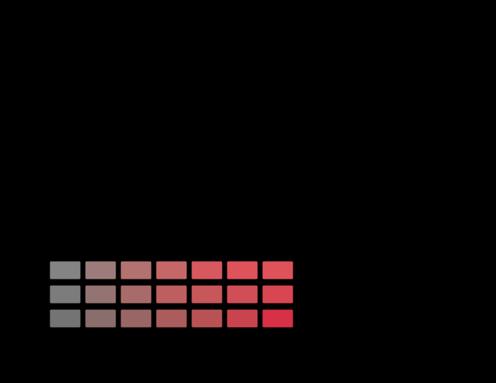
A gradient of one hue, mapped into a press's gamut 3 ways. Chroma asked for along the bottom, chroma delivered up the side, for a ramp at lightness 55 and hue angle 25°. A colorimetric intent follows the diagonal until the press runs out and is flat afterwards — the flat part is a gradient arriving as a single colour. The perceptual intent is under the diagonal from the start, which is the price of never going flat. What it takes to deliver it

A budget drawn through one hue

The three-stage error budget this collection publishes for a colour-management chain is computed over twenty-four colours of a single hue at a single lightness. The quantity that actually varies with hue — how many distinguishable colours a rendering intent destroys — runs from nothing at all to more than a third, and the hue the budget uses is near the bottom of that range.

Every census row under five constructions of the same test set. A slope chart with 5 columns — lattice, coarse, fine, uniform, natural — and one line per change of light in the census, each line joining that row's mean residual under each construction. Four of the five columns describe the same region of surfaces walked at different densities or against different measures; the last is the clamped, realistic family, which is not linear in its parameters and is therefore answering a slightly different question. The levels move: between the coarse and fine lattices every row shifts by seven to nine per cent, in the same direction, which is a common-mode factor no published residual here has ever carried. The order almost survives. Inside the region exactly one pair crosses, and it is the pair the standard error had already flagged; under the clamped set two more cross, including one the error separates by nearly nine standard errors. The crossing lines are drawn heavy. Where the model breaks

What the audit still cannot reach

Two rounds have now swept every declared width in this collection and one of its structural choices. Three structural choices remain, none of them has a multiplier to sweep, and the reason each resists is different — which makes the list a description of where this kind of audit ends rather than a queue of work.

What six of this collection's published numbers do when the unit changes. Six quantities, from six calculations that share nothing: a change of light after an observer has adapted, a camera profile's error, the gap between the two standard observers, a metameric pair under the lamp that breaks it, the same image on two papers, and an observer two seconds into a new room. Each is recomputed under all six units and every unit is calibrated onto ΔE2000's scale first, so the bar is not a change of units in the ordinary sense. The bar is the ratio of the largest reading to the smallest, and it runs from 1.71 to 2.30. Five of the six are printed in ΔE2000 by the essays that report them; the sixth is printed in CAM16-UCS, because the model it comes out of defines that unit. Where the model breaks

A choice with no magnitude

An audit can multiply a width by 1.25 and report an elasticity. It cannot multiply CIEDE2000 by anything. Auditing a structural choice needs a different instrument, and building one shows that six published numbers in this collection each carry a factor of about two of unit-choice — after the change of scale has been taken out.

The adaptation census in six units, calibrated onto one scale. Each line is one of the fourteen changes of light in the adaptation census, drawn across the six units the results could have been published in. Every unit is multiplied by the single factor that best carries it onto ΔE2000 over a reference sample of surface pairs, so the vertical axis means the same thing in every column and a sloping line is a disagreement rather than a change of scale. The levels move by up to a factor of two. More to the point, the lines cross: ΔEok puts 10 of the 91 pairs of rows in the other order, and CAM16-UCS, the only appearance unit here, puts the fewest — 2. What light is

The census in six units

Recomputing every change of light in the adaptation census under six colour-difference formulae, with the scale factor divided out, leaves a table whose levels move by up to a factor of three point seven. The rows that move most are the mild ones, which is the opposite of what a reader would guess and is a property of where each formula was fitted.

How far each unit is from being a rescaling of the one this collection publishes in. One row per unit on the menu. The bar is the root-mean-square scatter about that unit's own best rescaling of ΔE2000, over 374 pairs of surfaces differing by a fraction of a unit to about ten. A bar of zero would mean the unit is ΔE2000 in different money — every printed number would change and no conclusion would. ΔE2000's own row is zero by construction and is the check that the table is computed the right way round. The two units that divide a chroma difference by the chroma it was measured at, ΔE94 at 15 per cent and CAM16-UCS at 24, are closer to it than the three that do not, which run from 28 to 35. The split is by weighting and not by whether the unit is a matching difference or an appearance one. Difference and uniformity

The weighting is the disagreement

Five colour-difference formulae, three decades and two committees, and the single property that predicts which of them agree is whether a chroma difference gets divided by the chroma it was measured at. It sorts the menu exactly, it cuts across the distinction between a matching difference and an appearance one, and it halves the census's largest sensitivity.

The census along the line from ΔE76 to ΔE94, and past it. ΔE94 is ΔE76 with two weighting constants in it, and at zero those constants make every weight exactly one, so the two formulae are joined by a line rather than separated by a choice. The horizontal axis is how much of the published weighting is applied: 0 is exactly ΔE76, 1 is exactly ΔE94, and 3 is three times more weighting than anybody has proposed. The falling curve is the census's mean elasticity to how saturated its test set is, which drops from 1.11 to 0.74 — most of the fall happening before the published value is reached. The other curve is Kendall's τ against ΔE2000's ranking, and it peaks at w = 0.5, not at 1: the weighting that best reproduces the published ordering is about half the published weighting. There is no value of this dial that reaches ΔE2000, whose rotation term is not on this line at all. Difference and uniformity

A dial through a discrete menu

ΔE*94 is ΔE*ab with two weighting constants in it, and at zero those constants make every weight exactly one — so the two ends of the oldest disagreement in colour difference are joined by a line rather than separated by a choice. Walking it gives a derivative where a menu gives only a spread, and the derivative says the published weighting is on the far side of the interesting part.

463 essays on this thread, page 11 of 20 · all threads · all essays